Paula Moraga

<!--
poster arab-american
slides: 1,21-23,25-37,56
1-3,20-37,56-57

spatial statistics
disease
environment
-->

<style>

.pull-left-50 {
  float: left;
  width: 50%;
}
.pull-right-50 {
  float: right;
  width: 50%;
}

.pull-left-60 {
  float: left;
  width: 60%;
}
.pull-right-40 {
  float: right;
  width: 40%;
}

.pull-right-40-padding {
  float: right;
  width: 38%;
  padding-left: 10px
}

</style>

</style>

<div class = "content">
<br>
<center>
<div style = 'margin-top: -60px; margin-bottom: -100px; margin-left:-30px; margin-right:-30px;'>
<p class="text-center" style = 'font-size: 56px; line-height:1.5; font-weight:bold;'>Geospatial Data Science for Public Health Surveillance</p>

</div>
</center>

<br>

<div style = 'padding: 40px; padding-left: 40px; font-size: 32px; font-weight:bold; margin-top: 10px; margin-bottom: -50px;'>
<br>
Paula Moraga, Ph.D.<br>
</div>

<div style = 'padding: 40px; padding-left: 40px; font-size: 28px; margin-bottom: -60px;'>
Asst. Professor of Statistics
</div>
<div style = 'padding: 40px; padding-left: 40px; font-size: 28px; margin-bottom: -55px;'>
King Abdullah University of Science and Technology (KAUST), Saudi Arabia
</div>

<div style = 'padding: 40px; padding-left: 40px; font-size: 26px; line-height:1.5;margin-bottom: 40px;'>
<a href='http://twitter.com/Paula_Moraga_' target='_blank'> <i class='fa fa-twitter fa-fw'></i>&nbsp; @Paula_Moraga_</a><br>
<a href='https://Paula-Moraga.github.io/' target='_blank'> <i class='fa fa-globe fa-fw'></i>&nbsp; www.PaulaMoraga.com</a><br>

</div>

</td>
<td>

</td>
</tr>
</table>

</div>

<!--

#---

# Education

- **PhD Mathematics**, University of Valencia, 2012

#-- Comment (Extraordinary Doctoral Award) --

- **MSc Biostatistics**, Harvard University, 2011
- **BSc Mathematics**, University of Valencia, 2006    
   Erasmus Johannes Gutenberg University Mainz
   
<p style = 'margin-bottom: 50px;'></p>

]

.pull-right-30[
<img src="./figures/valencialogo.png" style="width:100%;"/>
<img src="./figures/harvardlogo.png" style="width:100%;"/>
]

# Experience

-->

<!--

#---

**BSc Mathematics**, University of Valencia, Johannes Gutenberg U. Mainz

#--

Openfinance

#--

Start PhD and collaboration with cancer registry

#--

**MSc Biostatistics**, Harvard University

#--

Harvard Medical School, Brigham and Women's Hospital, MUSC <br>
Google Summer of Code <br>
European Centre for Disease Prevention and Control (ECDC)

#--

**PhD Mathematics**, University of Valencia

#--

Lancaster University <br>
Harvard University <br>
London School of Hygiene and Tropical & Medicine <br>
Queensland University of Technology (QUT) <br>
Lancaster University <br>
University of Bath <br>

#--

**KAUST** Prof. Statistics and PI GeoHealth

&nbsp;&nbsp;&nbsp;&nbsp;&nbsp;&nbsp;&nbsp;<img src="./figures/Statistics at KAUST_Logo for digital use_small.png" height = "100" alt = "a png">&nbsp;&nbsp;&nbsp;&nbsp;&nbsp;&nbsp;&nbsp;
<img src="./figures/logogeohealth.png" height = "100" alt = "a png">

-->

<!--
#---
<div style="margin-top:-20px"></div>

# Who am I?

<table style="margin:20px; border-top:0; border-bottom:0; margin-bottom: -20px;">
<tr>
<td>
<p style="font-size:25px"><b>Paula Moraga, Ph.D.</b></p>
Assistant Professor of Statistics <br>for Public Health at KAUST<br><br>
PI Geospatial Statistics and Health Surveillance Research Group<br><br>
<img src="./figures/Statistics at KAUST_Logo for digital use_small.png" height = "120" alt = "a png">&nbsp;&nbsp;&nbsp;&nbsp;&nbsp;&nbsp;&nbsp;
<img src="./figures/logogeohealth.png" height = "120" alt = "a png">
</td>
<td style="width:40%">
<img class = "circular--square" src="./figures/paula.png" width = "200" alt = "a png"><br><br>
<a href='http://twitter.com/Paula_Moraga_' target='_blank'><i class='fa fa-twitter fa-fw'></i>&nbsp; @Paula_Moraga_</a><br>
<a href='https://Paula-Moraga.github.io/' target='_blank'><i class='fa fa-globe fa-fw'></i>&nbsp; www.PaulaMoraga.com</a><br>
</td>
</tr>
</table>

<br>

<i class='fa fa-map-marked-alt fa-fw'></i>&nbsp; Geospatial data analysis, statistical modeling<br>
<i class='fa fa-hospital fa-fw'></i>&nbsp; Spatial epidemiology, disease mapping, health surveillance<br>
<i class='fa fa-laptop fa-fw'></i>&nbsp; Development of R packages and interactive visualization applications<br>
<i class='fa fa-book fa-fw'></i>&nbsp; Author book Geospatial Health Data http://bit.ly/bookgeo<br>
<i class='fa fa-graduation-cap fa-fw'></i>&nbsp; PhD Mathematics, Valencia. Master's Biostatistics, Harvard<br>

-->

---
background-image: url(./figures/overview.png)
background-size: contain

<!--                
#---

## https://www.paulamoraga.com/book-geospatial/

.pull-left[
<center>
<img src="./figures/bookcover.jpg"  style="margin-top:-5px; margin-left:-10px; width:100%;"/>
</center>
]

]

-->

---

# Books

.pull-left[
<center>
<img src="./figures/bookcover.jpg"  style="margin-top:-5px; margin-left:-10px; width:100%;"/>
</center>
<small><small>
<a href="https://www.paulamoraga.com/book-geospatial/">https://www.paulamoraga.com/book-geospatial/</a>
</small></small>
]

.pull-left[
<center>
<img src="./figures/bookcoverspatial.jpg"  style="margin-top:-5px; margin-left:10px; width:100%;"/>
</center>
<small><small>
<a href="https://www.paulamoraga.com/book-spatial/">&nbsp;&nbsp;&nbsp; https://www.paulamoraga.com/book-spatial/</a>
</small></small>
]
                    
---

<h3>Geospatial Health Data: Modeling and Visualization with R-INLA and Shiny (2019)
<a href="https://www.paulamoraga.com/book-geospatial/">
http://www.paulamoraga.com/book-geospatial/
</a>
</h3>

- Manipulate and transform point, areal, raster data, create maps with R

- Fit and interpret Bayesian spatial, spatio-temporal models w/ INLA, SPDE

- Interactive viz, reproducible reports, dashboards, and Shiny apps

- Health examples (model disease risk and quantify risk factors in different settings) but methods also useful to analyze geospatial data in other fields

<!--

- Manipulate and transform point, areal and raster data,<br> and create maps with R

- Fit and interpret Bayesian spatial and spatio-temporal models with INLA and SPDE

- Interactive visualizations, reproducible reports, dashboards, and Shiny apps

- Model disease risk and quantify risk factors in different settings

- Health examples but methods useful to analyze georeferenced data in other fields such as ecology or criminology

-->

---

<h3>Spatial Statistics for Data Science: Theory and Practice with R
(2023)
<a href="https://www.paulamoraga.com/book-spatial/">
http://www.paulamoraga.com/book-spatial/
</a>
</h3>

- Statistical methods, modeling approaches, and visualizations to analyze spatial data using R

- **Spatial data**: types, retrieval, manipulation and visualization

- **Areal data**: spatial neighborhood matrices, autocorrelation, spatial models

- **Geostatistical data**: spatial interpolation methods, kriging, model-based geostatistics

- **Point patterns**: intensity estimation, clustering, LGCPs

- Reproducible examples in disease risk, air pollution, species distribution, crime mapping, real state analyses

]

.pull-right[
<center>
<img src="./figures/bookcoverspatial.jpg"  style="margin-top:0px; margin-left:-10px; width:95%;"/>
</center>
]

<!--
#---

# Ciencia de datos geoespaciales para la vigilancia de la salud p&uacute;blica

<br>

## Datos y m&eacute;todos geoespaciales
## Aplicaciones en enfermedades tropicales
## Software estad&iacute;stico
## Investigaci&oacute;n actual
-->

---

# Geospatial Data Science for<br> Public Health Surveillance

<br>

## Geospatial data and methods
## Case studies in disease mapping
## Statistical software
## Current research

---

# Geospatial data and methods

---
background-image: url(figures/snow-cholera-map-pump-top-margin.png)
background-size: contain

# John Snow's map of cholera, London, 1854

---
# Geospatial methods for disease surveillance

Geospatial methods use data on disease cases, individuals at risk, and risk factors
such as demographic and environmental factors to

- Understand geographic and temporal patterns
- Highlight areas of high risk and detect clusters
- Identify potential risk factors
- Measure inequalities
- Quantify the excess of disease risk close to a putative source
- Early detection of outbreaks

🗣 Maps and other visualizations enable to represent disease risk and risk factors, and interactive dashboards facilitate the communication of results

✍️ Results guide decision makers
to better allocate limited resources and
to design strategies for disease prevention and control

🌍 Many of these methods are also useful to analyze georeferenced data in others fields such as ecology, environment and criminology

---
background-image: url(figures/arealgeostatisticalpointpatterns.png)
background-size: contain
background-position: left 50%

# Types of spatial data

[Moraga and Lawson, Computational Statistics & Data Analysis, 2012](https://doi.org/10.1016/j.csda.2011.11.011)   
[Moraga et al., Parasites & Vectors, 2015](https://doi.org/10.1186/s13071-015-1166-x)   
[Moraga and Montes, Statistics in Medicine, 2011](https://doi.org/10.1002/sim.4160)

---
<div style="margin-top:-40px"></div>

# Areal data

**Standardized Mortality Ratio (SMR)** is often used to estimate disease risk

`$$SMR \mbox{ in area } i =
SMR_i = \frac{Y_i}{E_i} = \frac{\mbox{number observed cases in area } i}{\mbox{number expected cases in area } i}$$`

`$SMR_i = 1$` `$\rightarrow$` same number of cases observed as expected  
`$SMR_i > 1$` `$\rightarrow$` more number of cases observed than expected (high risk)
`$SMR_i < 1$` `$\rightarrow$` less number of cases observed than expected (low risk)

**Limitations**

SMRs may be misleading and unreliable in areas with small populations or rare diseases.
Models enable to incorporate covariates and borrow information from neighboring areas to obtain smoothed relative risks

---
<div style="margin-top:-40px"></div>

# Areal models

Model to estimate disease relative risk `$\theta_i$` in areas `$i=1,\ldots,n$`

`$$Y_i|\theta_i \sim Poisson(E_i \times \theta_i)$$`
`$$\log(\theta_i)  = \boldsymbol{z}_i \boldsymbol{\beta} + u_i + v_i$$`

- `$Y_i$`: number observed cases in area `$i$`
- `$E_i$`: number expected cases in area `$i$`
- `$\theta_i$`: relative risk in area `$i$`

Fixed effects quantify the effects of the covariates on the disease risk

- `$\boldsymbol{z}_i = (1, z_{i1}, \ldots, z_{ip})$` vector of the intercept and covariates   
`$\beta = (\beta_0, \beta_1, \ldots, \beta_p)'$` coefficient vector

Random effects represent residual variation which is not
explained by the available covariates

- `$u_i$`: structured spatial effect to account for the spatial
dependence between relative risks (areas that are close show
more similar risk than areas that are not close)
- `$v_i$`: unstructured spatial effect to account for independent noise

---

# Spatial neighborhood matrix

```r
library(spdep)

nb <- poly2nb(map)
```

```r
## [[1]]
## [1] 21 28 67
## 
## [[2]]
## [1]  3  4 10 63 65
```

---

# Inference using INLA

`$$Y_i|\theta_i \sim Poisson(E_i \times \theta_i)$$`
`$$\log(\theta_i)  = \boldsymbol{z}_i \boldsymbol{\beta} + u_i + v_i$$`

```r
library(INLA)

formula <- Y ~ cov +
  f(idareau, model = "besag", graph = g, scale.model = TRUE) +
  f(idareav, model = "iid")

res <- inla(formula, family = "poisson", data = map@data,
  E = E, control.predictor = list(compute = TRUE))

# Posterior mean and 95% CI
map$RR <- res$summary.fitted.values[, "mean"]
map$LL <- res$summary.fitted.values[, "0.025quant"]
map$UL <- res$summary.fitted.values[, "0.975quant"]
```

R-INLA: http://www.r-inla.org/

---
# Visualization

```r
library(leaflet)

pal <- colorNumeric(palette = "YlOrRd", domain = map$SIR)

leaflet(map) %>% addTiles() %>%
addPolygons(color = "grey", weight = 1, fillColor = ~ pal(SIR)) %>%
addLegend(pal = pal, values = ~SIR, title = "SIR")
```

---
<div style="margin-top:-10px"></div>

# Geostatistical data

---
<div style="margin-top: -45px;">

# Geostatistical models

Models to predict prevalence at unsampled locations

`$$Y_i|P(\boldsymbol{x}_i)\sim \mbox{Binomial} (n_i, P(\boldsymbol{x}_i))$$`
`$$\mbox{logit}(P(\boldsymbol{x}_i))  = \boldsymbol{z}_i \boldsymbol{\beta} + S(\boldsymbol{x}_i) + u_i$$`

`$Y_i$` number people positive, `$n_i$` number people tested, `$P(x_i)$` prevalence at `$\boldsymbol{x}_i$`

Covariates based on characteristics known to affect disease transmission
(temperature, precipitation, vegetation, elevation, population density, etc.)

Random effects model residual variation not explained by covariates

---

# Triangulated mesh for SPDE approach

```r
library(INLA)

mesh <- inla.mesh.2d(
  loc = coo, offset = c(50, 100),
  cutoff = 1, max.edge = c(30, 60))
```

---

# Spatial covariates

```r
library(raster)

r <- getData(name = "alt", country = "GMB", mask = TRUE)
```

---

# Inference using INLA and SPDE

`$$Y_i|P(\boldsymbol{x}_i)\sim \mbox{Binomial} (n_i, P(\boldsymbol{x}_i))$$`
`$$\mbox{logit}(P(\boldsymbol{x}_i))  = \boldsymbol{z}_i \boldsymbol{\beta} + S(\boldsymbol{x}_i) + u_i$$`

```r
library(INLA)

formula <- y ~ 0 + b0 + alt + f(s, model=spde) + f(idu, model="iid")

res <- inla(formula, family = "binomial", Ntrials = numtrials,
  control.family = list(link = "logit"),
  data = inla.stack.data(stk.full),
  control.predictor = list(compute = TRUE, link = 1,
                           A = inla.stack.A(stk.full)))

index <- inla.stack.index(stack = stk.full, tag = "pred")$data

# Posterior mean and 95% CI
prev_mean <- res$summary.fitted.values[index, "mean"]
prev_ll <- res$summary.fitted.values[index, "0.025quant"]
prev_ul <- res$summary.fitted.values[index, "0.975quant"]
```

<!--
#---
<div style="margin-top:-40px"></div>

# Point patterns

Assume point pattern `$\{s_i: i=1, \ldots, n\}$` has been generated as a realization of a point process
`$Z = \{Z(s): s \in \mathbb{R}^2\}$`

Point processes are stochastic models that describe the locations of events of interest and possibly some additional information such as marks that inform about different types of events (e.g., cases and controls)

A point process model can be used to identify patterns in the distribution of the observed locations, estimate the intensity of events, and learn about the correlation between the locations and spatial covariates

#---

# Point process models

**Homogeneous Poisson process**

- Number of events in any region `$A$` distributed as `$\mbox{Poisson}(\lambda |A|)$`<br> where `$\lambda$` constant value denoting the intensity and `$|A|$` area of `$A$`
- Number of events in disjoint regions are independent
- Thus, an event is equally likely to occur at any location within the study region, regardless of the locations of other events

**Log-Gaussian Cox process (LGCP)**

- Poisson process with a varying intensity which is itself a stochastic process `$\Lambda(s) = exp(Z(s))$`, `$Z = \{Z(s): s \in \mathbb{R}^2\}$` Gaussian process
- Conditional on `$\Lambda(s)$`, LGCP is a Poisson process with intensity `$\Lambda(s)$`
- Thus, the number of events in any region `$A$` distributed as `$\mbox{Poisson}(\int_A \Lambda(s)ds)$` and the event locations are an independent random sample from the distribution on `$A$` with probability density proportional to `$\Lambda(s)$`

#---

# Log-Gaussian Cox process

Locations are a realization of a LGCP with varying intensity which is a stochastic process `$\Lambda(s)= exp(\eta(s))$`, `$\eta = \{\eta(s): s \in \mathbb{R}^2\}$` Gaussian process

Fit model by approximating using a gridding approach:

- Discretize study region into a grid `$\{s_{ij}\}$` with `$n_1 \times n_2$` cells

- Mean number of events in cell `$s_{ij}$` is `$\Lambda_{ij}=\int_{s_{ij}} exp(\eta(s))ds \approx |s_{ij}| exp(\eta_{ij})$`,
where `$|s_{ij}|$` is the cell area

- Number of events in cell `$s_{ij}$` are independent and Poisson distributed

`$$y_{ij}|\eta_{ij} \sim Poisson(|s_{ij}| exp(\eta_{ij}))$$`
`$$\eta_{ij} = \beta_0 + \beta_1 \times cov(s_{ij}) + f_s(s_{ij}) + f_u(s_{ij})$$`

#---

# Computational grid

Discretize study region into a grid and count the number of points in each cell

```r
library(rnaturalearth)
library(raster)

# Retrieve study region boundaries
map <- ne_countries(type = "countries", country = country)

# Create raster grid
resolution <- 0.1
r <- raster(map, resolution = resolution)

# Number points in each cell
r[] <- 0
tab <- table(cellFromXY(r, dpts))
r[as.numeric(names(tab))] <- tab

# Grid to be passed to INLA
grid <- rasterToPolygons(r)
```

#---

# Inference using INLA

`$$y_{ij}|\eta_{ij} \sim Poisson(|s_{ij}| exp(\eta_{ij}))$$`
`$$\eta_{ij} = \beta_0 + \beta_1 \times cov(s_{ij}) + f_s(s_{ij}) + f_u(s_{ij})$$`

```r
library(INLA)

formula <- Y ~ 1 + cov +
  f(id, model = "rw2d", nrow = nrow, ncol = ncol) +
  f(id2, model = "iid")

res <- inla(formula, family = "poisson", data = grid@data,
            E = cellarea, control.predictor = list(compute = TRUE))

# Posterior mean number of events and 95% CI
grid$NE <- res$summary.fitted.values[, "mean"] * cellarea
grid$LL <- res$summary.fitted.values[, "0.025quant"] * cellarea
grid$UL <- res$summary.fitted.values[, "0.975quant"] * cellarea
```

-->

---
class: inverse

<br>

# Geospatial Models for Disease Mapping

<br>

## Lymphatic filariasis in sub-Saharan Africa

## Leptospirosis in Brazil

## COVID-19 in Colombia

<!--
#---
class: inverse, center, middle

# Lymphatic filariasis in sub-Saharan Africa

### Modelling the distribution and transmission intensity of lymphatic filariasis in sub-Saharan Africa prior to scaling up interventions: integrated use of geostatistical and mathematical modelling

### [Moraga, et al., Parasites & Vectors, 8:560, 2015](https://doi.org/10.1186/s13071-015-1166-x)

-->

---

# Geospatial modelling of lymphatic filariasis prevalence in sub-Saharan Africa

Lymphatic filariasis (LF) caused by microscopic worms and transmitted by mosquitoes

Disfigurement and disabilities due to lymphedema, elephantiasis and hydrocele

]

<img src="./figures/lfAedesaegypti.jpg" style="width:80%;"/>
<img src="./figures/lfsymptoms1.jpg" style="width:80%;"/>
]

---
background-image: url(./figures/lfburdenourworldindata1.png)
background-size: contain

&nbsp;&nbsp;&nbsp;&nbsp;&nbsp;&nbsp;&nbsp;&nbsp;&nbsp;&nbsp; Main strategy against the disease is Mass Drug Administration.<br>
Resources are limited and need to decide which are the areas most in need.

<!--
#---
<div style="margin-top:-20px"></div>

# Geospatial modelling of lymphatic filariasis prevalence in sub-Saharan Africa

Main strategy against the disease is **Mass Drug Administration**
(recommended to entire populations in regions where prevalence
exceeds 1% annually for at least five years)

Resources are limited and need to decide which are the areas most in need

-->

<!--
https://cntd.lstmed.ac.uk/our-work/themes/mass-drug-administration-mda

https://ourworldindata.org/grapher/prevalence-of-lymphatic-filariasis

https://apps.who.int/iris/bitstream/handle/10665/250245/WER9139.pdf;jsessionid=BFDC2323CD77FB87F3856DF837A3B468?sequence=1

https://ig.ft.com/special-reports/elephantiasis/
-->

<!--
#---
<div style="margin-top:-10px"></div>

# LF prevalence surveys in sub-Saharan Africa

<!--

<div style="width:20%;">
3197 surveys 1990-2014
</div>
<div style="width:30%; margin-left:-50px; margin-bottom:-180px">
<img src="./figures/lficttest.jpg" style="width:100%;"/>
</div>

-->

---
<div style="margin-top:-30px"></div>

# Geospatial modelling of lymphatic filariasis prevalence in sub-Saharan Africa

3197 LF prevalence surveys, 1990-2014

---
<div style="margin-top: -35px;">

# Predict local LF prevalence

`$$Y_i|P(\boldsymbol{x}_i)\sim \mbox{Binomial} (n_i, P(\boldsymbol{x}_i))$$`
`$$\mbox{logit}(P(\boldsymbol{x}_i))  = \boldsymbol{z}_i \boldsymbol{\beta} + S(\boldsymbol{x}_i) + u_i$$`

Covariates based on characteristics known to affect LF transmission
(precipitation, vegetation, elevation, land cover, population density, etc.)

Random effects model residual variation not explained by covariates

---
background-size: contain

###  Maps can help surveillance activities by

### - identifying areas that require enhanced interventions
### - setting a benchmark for evaluating the impact of interventions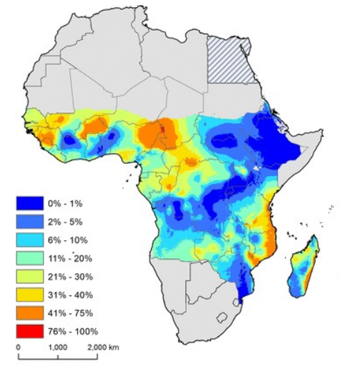

]

![](./figures/africaLF.png)

]

[Moraga, et al., Parasites & Vectors, 2015](https://doi.org/10.1186/s13071-015-1166-x)

<!--
#---
class: inverse, center, middle

# Leptospirosis in Brazil

### Spatio-temporal determinants of urban leptospirosis transmission: Four-year prospective cohort study of slum residents in Brazil

### [Hagan, Moraga, et al., PLOS Neglected Tropical Diseases,<br> 10(1): e0004275, 2016](https://journals.plos.org/plosntds/article?id=10.1371/journal.pntd.0004275)

-->

---

# Spatio-temporal determinants of urban leptospirosis transmission in Brazil

**Transmission** via direct skin or mucosal contact with animal reservoirs or an environment contaminated with infected  urine

**Manifestations**: fever, headache, myalgia, aseptic meningitis, jaundice, renal failure, pulmonary hemorrhage syndrome

Urban health problem due to the **rapid and disorganized expansion of urban centers**, creating ecological conditions for rat-borne transmission

Predominantly affects **vulnerable populations** such as subsistence farmers and residents of urban<br> slums in the tropics

]

.pull-right-50[
<img src="./figures/cyclelepto.jpg" style="margin-top:10px; padding-left:20px; width:90%;"/>
]

---

# Leptospirosis in Pau da Lima, Brazil

Pau da Lima is a urban slum in Salvador, Bahia, that hosts a densely populated community with a high annual incidence of leptospirosis

---

---

# Leptospirosis in Pau da Lima
<div style="margin-top: -10px;">

**Objective**:
Understanding the spatio-temporal patterns of leptospirosis and identifying targets for intervention in Pau da Lima

**Data**:
2003 subjects recruited and followed for a four-year period (2003-2007).
Annual administration of questionnaires and GIS mapping to determine socio-behavioral and environmental risk factors.

### Spatio-temporal mixed model
<div style="margin-top: -10px;">

`$$Y_{ij}| P(\boldsymbol{s}_i, j) \sim Bernoulli(P(\boldsymbol{s}_i, j))$$`

`$$logit(P(\boldsymbol{s}_i, j))=
\boldsymbol{z}_{ij} \boldsymbol{\beta}  + \xi(\boldsymbol{s}_i,j) + u_i$$`

`$$\xi(\boldsymbol{s}_i,j)=a \xi(\boldsymbol{s}_i,j-1)+w(\boldsymbol{s}_i,j)$$`

`$$|a|<1, \xi(\boldsymbol{s}_i,1) \sim N(0, \sigma_w^2/ (1-a^2)),
w(\boldsymbol{s}_i,j) \sim N(0,\sigma^2_w C(h))$$`

`$$u_i \sim N(0, 1/\tau_u)$$`

<br>
[Hagan, et al., PLOS Neglected Tropical Diseases, 2016](https://journals.plos.org/plosntds/article?id=10.1371/journal.pntd.0004275)

---
background-image: url(./figures/variables.png)
background-size: contain

<!--
#---

# Selection fixed effects

Within each group, fit GAM using all categorical variables, non-linear effects of continuous variables, and  interactions between them

Remove covariates one by one until obtaining a model with minimum AIC

- Demographic and social status factors `$\longrightarrow$` V1
- Health factors `$\longrightarrow$` V2
- Occupational exposures `$\longrightarrow$` V3
- Household environment `$\longrightarrow$` V4
- Household behaviour `$\longrightarrow$` V5
- Household reservoirs `$\longrightarrow$` V6
- Work behaviour `$\longrightarrow$` V7
- Work reservoirs `$\longrightarrow$` V8

Merge groups and explore further simplification by backward elimination until it is no longer possible to reduce AIC

V1+V2+V3+V4+V5+V6+V7+V8 `$\longrightarrow$` V

-->

<!--
#---

# Selection fixed effects

Model includes:

- year of follow-up (1st, 2nd, 3rd or 4th year)
- gender (male/ female)
- being literate (literate / illiterate)
- house elevation
- observation of rats near house (observe/ not observe)
- contact with mud near house (contact / no contact)
- non-linear effect of age

-->

---

# Risk factors

<!--
#---

# Areas with highest (red) and lowest (blue) odds of infection

-->

---
<div style="margin-top:-20px;">
<h1>High-risk region</h1> 
<p style="margin-top:-20px; margin-bottom:20px;">High-risk region in which measured risk is consistent with prediction <p>
</div>

---
<div style="margin-top:-20px;">
<h1>High positive residual</h1> 
<p style="margin-top:-20px; margin-bottom:20px;">Poor household construction and flood risk due to poor infrastructure <p>
</div>

---
<div style="margin-top:-20px;">
<h1>High negative residual</h1> 
<p style="margin-top:-20px; margin-bottom:20px;">Open sewers with structural barriers to stop overflow <p>
</div>

</style>

<!--
#---

# Conclusions

<br>

- Young adults, males, and individuals with low social status may have
activities that place them in more frequent or more intense contact
with sources of transmission

- Interventions such providing adequate sanitation systems may reduce
the burden of leptospirosis by protecting residents from contact with
contaminated soil and mud during heavy rain events

- Areas in which transmission risk cannot be adequately explained using
known risk factors enable the identification of new hypotheses about
transmission and guide targeted interventions

-->

---

# Spatio-temporal prediction of COVID-19 in Cali, Colombia, by integrating compartment and point process models

[Ribeiro Amaral, et al. SERRA, 2022](https://doi.org/10.1007/s00477-022-02354-4)

---
<div style="margin-top:-20px"></div>

# SIR + LGCP model

Two-step approach:

Aggregate data in the whole region for each time.
Fit temporal SIR (Susceptible, Infected, Recovered) compartment model to obtain the predicted number of infectious individuals at each time
`$$\begin{align*}
    \frac{dS(t)}{dt} &= -\beta S(t) \frac{I(t)}{N} \\
    \frac{dI(t)}{dt} &= +\beta S(t) \frac{I(t)}{N} - \gamma I(t) \\
    \frac{dR(t)}{dt} &= +\gamma I(t)
\end{align*}$$`
Number of individuals in the population `$S(t) + I(t) + R(t) = N$` constant

Disease parameters: `$\beta > 0$` infectious rate, `$\gamma > 0$` recovery or death rate

We extend SIR model to allow for the incorporation of age-stratified contact information, which provides valuable information for decision-making

SIR model could be extended to consider more compartments (e.g.,<br> `$I_S(t)$` symptomatic, `$I_A(t)$` asymptomatic)

---
<div style="margin-top:0px"></div>

# SIR + LGCP model

Fit a log-Gaussian Cox process for the locations of infected individuals in the studied region and time, with mean depending on the predicted number of infected people at that time obtained from the SIR model

<br>

`$$\begin{align}
    N(A, t) &\sim \text{Poisson}\left(\int_{A}\Lambda(\mathbf{x}, t)d\mathbf{x}\right) \\
    \Lambda(\mathbf{x}, t) &= \lambda_{0}(\mathbf{x}, t)\ I(t)\ \exp(S({\mathbf{x}, t})) \nonumber \\
\end{align}$$`
`$$\begin{align}
\lambda_{0}(\mathbf{x}, t):\ &\text{Proportional to the population density and integrates to 1}\\
I(t):\ &\text{Number of infected people at time } t\ \text{obtained from SIR model}\\
S(\mathbf{x}, t):\ &\text{Spatial Gaussian random field with Matern covariance function} \nonumber \\
\end{align}$$`

---

# COVID-19 prediction in Cali, Colombia

4518 COVID-19 locations from 21/1/2020 to 18/6/2020

Using simulations and real COVID-19 data, we showed
SIR+LGCP model has better forecasting performance than other LGCP models that do not do use information from the SIR model

SIR+LGCP model can help decision-makers to identify high-risk locations and vulnerable populations to develop better strategies for infectious diseases prevention and control

---
class: inverse, center, middle

# Statistical software

---
background-image: url(./figures/overviewsoftware2.png)
background-size: contain

# Statistical software

<div style="color: gray; height: 20px;bottom:100px;left: 80px;position: fixed;">
<br><br>
<a href='https://f1000research.com/articles/7-1374/v3' target='_blank'>Moraga, et al. F1000 Research, 7:1374, 2019</a><br>
<a href='https://doi.org/10.1016/j.sste.2017.08.001' target='_blank'>Moraga. Spatial and Spatio-temporal Epidemiology, 23:47-57, 2017</a><br>
</div>

---
<div style="margin-top:-40px"></div>

# SpatialEpiApp

Shiny app for disease risk estimation, cluster detection, and interactive viz

- Risk estimates by fitting Bayesian models with [INLA](http://www.r-inla.org/)
- Detection of clusters by using the scan statistics in [SaTScan](https://www.satscan.org/)

http://www.paulamoraga.com/software/

```r
library(devtools)
install_github("Paula-Moraga/SpatialEpiApp")
library(SpatialEpiApp)
run_app()
```

---
<div style="margin-top:-30px"></div>

<b>Upload map and data<b>

<b>Bayesian disease risk models
&nbsp;&nbsp;&nbsp;&nbsp;&nbsp;&nbsp;
Scan statistics for detection of clusters<b>

---

# epiflows. Travel-related spread of disease

<div style="color: gray; height: 30px;bottom:10px;left: 80px;position: fixed;">
<a href='https://f1000research.com/articles/7-1374/v3' target='_blank'>Moraga, et al. F1000 Research, 7:1374, 2019</a><br>
</div>

Mathematical model that predicts the number of cases that could be spread to other locations from an infectious location together with uncertainty measures

Integrates information about the number of infectious cases, population flows, lengths of stay, incubation and infectious periods

---

**Total infections introduced in O from S = Exportations + Importations**

**Exportations**
`$$E_{S,O}= C_{S,W} \times p_O \times p_i$$`
- `$C_{S,W}$` cumulative number of infections in location `$S$` and time window `$W$`
- `$p_O = \frac{T_{S,O}^W}{pop_S}$` per capita probability that a resident of `$S$` travels to `$O$`
- `$T_{S,O}^W$` residents of `$S$` travelling to `$O$`. `$pop_S$` population `$S$`
- `$p_i = min\left(\frac{D_E+D_I}{W}, 1\right)$` prob. infection incubated or infectious during `$W$`

**Importations**
`$$I_{S,O} = T_{O,S}^W \times \lambda_S \times p_l$$`
- `$T_{O,S}^W$` number travelers visiting `$S$` from `$O$` in time window `$W$`
- `$\lambda_S = \frac{C_{S,W}\times L_0}{pop_S \times W}$` per capita risk infection of travelers visiting `$S$` during stay
- `$L_0$` average length of stay
- `$p_l = min\left(\frac{D_E+D_I}{L_0}, 1\right)$` prob. return home while incubating or infectious

**Uncertainty** obtained by sampling from incubation `$D_E$` and infectious `$D_I$` period distributions. This produces a full distribution for `$p_i$` and `$p_l$`, and in turn to exportations, importations, and total number of infections

<!--
#---
background-image: url(./figures/recon.png)
background-size: contain

<div style="color: gray; height: 20px;bottom:70px;left: 80px;position: fixed;">
<br><br>
<a href='https://www.repidemicsconsortium.org/' target='_blank'>https://www.repidemicsconsortium.org/</a><br>
</div>

#---

&nbsp;&nbsp;&nbsp;&nbsp;&nbsp;&nbsp; https://afrimapr.github.io/afrimapr.website/

-->

---

# Current Research

## Statistical methods and computational tools to solve challenging problems and improve population health

## 1. Precision disease mapping
## 2. Digital health surveillance
## 3. Interactive visualization apps

---

# 1. Precision disease mapping

---

# Disease mapping

Disease maps help decision-makers to target health interventions and directing resources where most needed

Map shows malaria prevalence in Mozambique.

Area-level data unable to show how disease risk varies within areas

Areal estimates make difficult targeting health interventions and directing resources where most needed

]

[Moraga, et al., Spatial Statistics, 2017](https://doi.org/10.1016/j.spasta.2017.04.006)

[Zhong and Moraga, JABES, 2023](https://doi.org/10.1007/s13253-023-00559-w)

---

# Disaggregate area-level data

High-resolution estimates permit to
find differences in disease risk within study regions, and
identify areas and groups of people at higher risk

---
background-image: url(./figures/regressionrescov.png)
background-size: contain
background-position: 0 250px

# Spatially misaligned data

Quantifying risk factors with misaligned data.
Investigate relationship between a response variable and explanatory variables available at different spatial scales
(e.g., lung cancer at county level and smoking at state level)

https://vizhub.healthdata.org/subnational/usa

---
class: inverse, center, middle

# 2. Digital health surveillance

---

# Disease surveillance systems

Disease surveillance systems are critical to early detection of epidemics and the design of control
strategies

Traditional surveillance systems rely on data gathered with a considerable delay and
make surveillance systems ineffective for real-time surveillance

<br>

---

# Digital data sources

Real-time digital information may enable to detect outbreaks earlier

<br>

<span style="color: gray">"Flu plus fever, not a good way to start the weekend"</span>

<br>

<span style="color: gray">"I'm so irritated at this cough and fever"</span>

<br>

<span style="color: gray">"This flu, fever & throat ache won't let me sleep"</span>

</center>

---
# Demographic and environmental risk factors

<!--

## Existing approaches do not produce inferences at spatial resolutions actionable by policymakers

</center>

[The New York Times, 2008](https://www.nytimes.com/),
[Yang et al., 2015, PNAS](https://doi.org/10.1073/pnas.1515373112),
[HealthMap, 2018, PNAS](http://www.healthmap.org/en/)

-->

---

# Digital health surveillance system

- **Data-gathering platform**
- **Modelling framework** that integrates multiple data sources so as to produce local probabilistic predictions of disease activity in real-time
- **Interactive dashboard** that alert public health officials when
elevated disease levels are anticipated, and provide insights about disease drivers

<!--
- display of current and historical disease patterns
- disease predictions
- notifications of outbreaks
- reports summarizing disease level
- overlay of maps with contextual information

# Disease surveillance system into practice
  
 - System portable and accessible by health departments worldwide
 
- Put the surveillance system into practice by collaborating with national and international partners

- This information will be used to respond to public health threats in a timely and appropriate manner

Integrates the data-gathering platform, the modelling architecture and a dashboard including interactive data visualizations and reports
-->

---
class: inverse, center, middle

# 3. Development of interactive visualization applications for policymaking

---

# Interactive visualizations for policymaking

<div style="color: gray; height: 30px;bottom:10px;left: 80px;position: fixed;">
<a href='https://doi.org/10.1016/j.sste.2017.08.001' target='_blank'>Moraga. Spatial and Spatio-temporal Epidemiology, 23:47-57, 2017</a><br>
</div>

Effective communication and proper and timely dissemination of information for the development and implementation of population health policies

- Digital web health atlases (cancer, cardiovascular, infectious diseases)
- Digital health surveillance systems to monitor diseases in real-time

![](./figures/animation.gif)

<a href="https://paulamoraga.shinyapps.io/spatialepiapp/">
https://paulamoraga.shinyapps.io/spatialepiapp/</a>

<!--
#---
background-image: url(./figures/kaustpositions-fellowship.png)
background-size: contain

-->

---
background-image: url(./figures/Admissions-com-2020-COVID.png)
background-size: contain
background-position: top right

# Join my research group at KAUST!

**KAUST** is an international research university located on the shores of the Red Sea in Saudi Arabia. KAUST is dedicated to advancing science and technology through interdisciplinary research, education and innovation.

**KAUST Fellowship**. All admitted students receive free tuition, annual living allowance, free housing, medical and dental coverage, relocation support

### KAUST http://kaust.edu.sa

### Statistics Program http://stat.kaust.edu.sa

### Admissions http://admissions.kaust.edu.sa

---
background-image: url(./figures/Admissions-com-2020-COVID.png)
background-size: contain
background-position: top right

# Join my research group at KAUST!

I am looking for outstanding PhD students and Postdocs to join my group

👩‍💻 Potential research areas include the development of innovative statistical and computational methods for health and environmental applications

- Disease mapping, cluster detection, early detection of outbreaks
- Integration of spatial and spatio-temporal data
- Development of R packages for data analysis and visualization

💪 Work closely with collaborators at KAUST and around the world

✈️ Generous travel funding for conferences and collaborative work

✨ Excellent research environment. Superb equipment and research facilities

<a href='http://twitter.com/Paula_Moraga_' target='_blank'> <i class='fa fa-twitter fa-fw'></i>&nbsp;@Paula\_Moraga_</a>&nbsp;&nbsp;&nbsp;&nbsp;&nbsp;
<a href='https://Paula-Moraga.github.io/' target='_blank'> <i class='fa fa-globe fa-fw'></i>&nbsp;www.PaulaMoraga.com</a>
&nbsp;&nbsp;&nbsp;&nbsp;&nbsp;
<a href='https://www.kaust.edu.sa/en' target='_blank'> <i class='fa fa-graduation-cap fa-fw'></i>&nbsp;www.kaust.edu.sa</a><br>

---

# References

<small>

Ribeiro Amaral, A., et al. (2022).
Spatio-temporal modeling of infectious diseases by integrating compartment and point process models. *SERRA*, 37, 1519-1533

Moraga, P., et al. (2019). epiflows: an R package for risk assessment of travel-related spread of disease. *F1000Research*, 7:1374

Moraga, P. (2018). Small Area Disease Risk Estimation and Visualization Using R. *The R Journal*, 10(1):495-506

Moraga, P. (2017). SpatialEpiApp: A Shiny Web Application for the analysis of Spatial and Spatio-Temporal Disease Data. *Spatial and Spatio-temporal Epidemiology*, 23:47-57

Moraga, P., et al. (2017). A geostatistical model for combined analysis of point-level and area-level data using INLA and SPDE. *Spatial Statistics*, 21:27-41

Hagan, J. E., Moraga, P., et al. (2016). Spatio-temporal determinants of urban leptospirosis transmission: Four-year prospective cohort study of slum residents in Brazil. *PLOS Neglected Tropical Diseases*, 10(1): e0004275

Moraga, P., et al. (2015). Modelling the distribution and transmission intensity of lymphatic filariasis in sub-Saharan Africa prior to scaling up interventions: integrated use of geostatistical and mathematical modelling. *Parasites & Vectors*, 8:560

]

.pull-right-30[
<img src="./figures/bookcoverspatial.jpg" style="width:80%; padding-left:30px;"/>
<br>
<img src="./figures/bookcover.jpg" style="width:80%; padding-left:30px;"/>
]

</small>

---

<div style = 'margin-top: 60px; margin-bottom: 40px;'>
<span style = 'font-size: 68px; line-height:1.5; font-weight:bold'>
Thanks!<br>
</span>
</div>

<span style = 'font-size: 38px; font-weight:bold'>
Paula Moraga<br>
</span>

<br>

<span style = 'font-size: 28px; line-height:1.5'>
<a href='http://twitter.com/Paula_Moraga_' target='_blank'> <i class='fa fa-twitter fa-fw'></i>&nbsp; @Paula_Moraga_</a><br>
<a href='https://Paula-Moraga.github.io/' target='_blank'><i class='fa fa-globe fa-fw'></i>&nbsp; www.PaulaMoraga.com</a><br>
</span>

</td>
<td>

</td>
</tr>
</table>

</div>