Bayesian spatial models. Spatial modeling of housing prices
Paula Moraga, KAUST
Materials based on the book Geospatial Health Data (2019, Chapman & Hall/CRC)
http://www.paulamoraga.com/book-geospatial
1 Bayesian spatial models
Bayesian hierarchical models (Banerjee, Carlin, and Gelfand 2004) can be used to analyze areal data that arise when an outcome variable is aggregated into areas that form a partition of the study region. Models can be specified to describe the variability in the response variable as a function of a number of covariates known to affect the outcome, as well as random effects to model residual variation not explained by the covariates. This provides a flexible and robust approach that allows us to assess the effects of explanatory variables, accommodate spatial autocorrelation, and quantify the uncertainty in the estimates obtained.
A commonly used spatial model is the Besag-York-Mollié (BYM) model (Besag, York, and Mollié 1991). Let us assume that \(Y_i\) are observed outcomes at regions \(i=1,\ldots,n\) that can be modeled using a Normal distribution. The BYM model is specified as
\[Y_i \sim Normal(\mu_i, \sigma^2), i = 1,\ldots,n,\] \[\mu_i = \boldsymbol{z_i \beta} + u_i + v_i.\]
Here, the fixed effects \(\boldsymbol{z_i \beta}\) are expressed using a vector of intercept and \(p\) covariates corresponding to area \(i\), \(\boldsymbol{z_i} = (1, z_{i1}, \ldots, z_{ip})\), and a coefficient vector \(\boldsymbol{\beta} = (\beta_0, \ldots, \beta_p)'\).
The model includes a spatial random effect \(u_i\) that accounts for the spatial dependence between outcomes indicating that areas that are close to each other may have similar values, and an unstructured exchangeable component \(v_i\) to model uncorrelated noise. The spatial random effect \(u_i\) can be modeled with an intrinsic conditional autoregressive model (CAR) that smooths the data according to a certain neighborhood structure. Specifically, \[u_i| \boldsymbol{u_{-i}} \sim N\left(\bar u_{\delta_i}, \frac{\sigma_u^2}{n_{\delta_i}}\right),\] where \(\bar u_{\delta_i}= n_{\delta_i}^{-1} \sum_{j \in \delta_i} u_j\), with \(\delta_i\) and \(n_{\delta_i}\) representing, respectively, the set of neighbors and the number of neighbors of area \(i\). The unstructured component \(v_i\) is modeled as independent and identically distributed normal variables with zero mean and variance \(\sigma_v^2\), \(v_i \sim N(0, \sigma_v^2).\)
2 Bayesian inference with INLA
Bayesian hierarchical models can be fitted using a number of approaches such as integrated nested Laplace approximations (INLA) (Håvard Rue, Martino, and Chopin 2009) and Markov chain Monte Carlo (MCMC) methods (Gelman et al. 2013). INLA is a computational approach to perform approximate Bayesian inference in latent Gaussian models. This includes a wide range of models such as generalized linear mixed models and spatial and spatio-temporal models. INLA uses a combination of analytical approximations and numerical integration to obtain approximated posterior distributions of the parameters and is very fast compared to MCMC methods.
The R-INLA package (Havard Rue, Lindgren, and Teixeira Krainski 2022) can be used to fit models using INLA. The INLA website (http://www.r-inla.org) includes documentation, examples, and other resources about INLA and the R-INLA package, including books that provide an introduction to Bayesian data analysis using INLA as well as practical examples in a variety of settings (Wang, Ryan, and Faraway 2018; Krainski et al. 2019; Moraga 2019; Gomez-Rubio 2020).
To install R-INLA, we use the install.packages() function specifying the R-INLA repository since the package is not on CRAN.
install.packages("INLA",
repos = "https://inla.r-inla-download.org/R/stable", dep = TRUE)
library(INLA)
Then, to fit a model, we write the linear predictor as a formula object in R,
and call the inla() function passing the formula, the family distribution, the data, and other options.
The object returned by inla() contains the fitted model. This object can be inspected,
and the posterior distributions can be post-processed using a set of functions provided by R-INLA.
R-INLA also provides functionality to specify priors, as well as to obtain a number of criteria that allow us to assess and compare Bayesian models such as the deviance information criterion (DIC) (Spiegelhalter et al. 2002), the Watanabe-Akaike information criterion (WAIC) (Watanabe 2010), and the conditional predictive ordinate (CPO) (Held, Schrödle, and Rue 2010).
3 Spatial modeling of housing prices in Boston, USA
Here, we provide an example on how to specify and fit a Bayesian hierarchical model to estimate housing prices in Boston, USA, using the R-INLA package.
3.1 Data
The Boston housing prices are in the spData package (Bivand, Nowosad, and Lovelace 2022), and can be obtained with the st_read() function of the sf package (Pebesma 2022) as follows.
library(sf)
library(spData)
map <- st_read(system.file("shapes/boston_tracts.shp", package = "spData"),
               quiet = TRUE)
This dataset contains housing data of 506 Boston census tracts including median prices of owner-occupied housing in USD 1000 (MEDV), per capita crime (CRIM), and average number of rooms per dwelling (RM).
We create the variable called vble with the logarithm of the median prices, and map this variable using mapview (Figure 3.1). The map suggests that the housing prices are greater in the west, and prices are related to those in neighboring areas.
map$vble <- log(map$MEDV)
library(mapview)
mapview(map, zcol = "vble")
Figure 3.1: Logarithm of housing prices in Boston per census tract from the spData package.
We will model the logarithm of the median prices using as covariates the per capita crime (CRIM) and the average number of rooms per dwelling (RM).
Figure 3.2 shows the relationships between pairs of variables visualized using the ggpairs() function of the GGally package (Schloerke et al. 2021).
We observe a negative relationship between the logarithm of housing price and crime, and a
positive relationship between the logarithm of housing price and the average number of rooms.
library(GGally)
ggpairs(data = map, columns = c("vble", "CRIM", "RM"))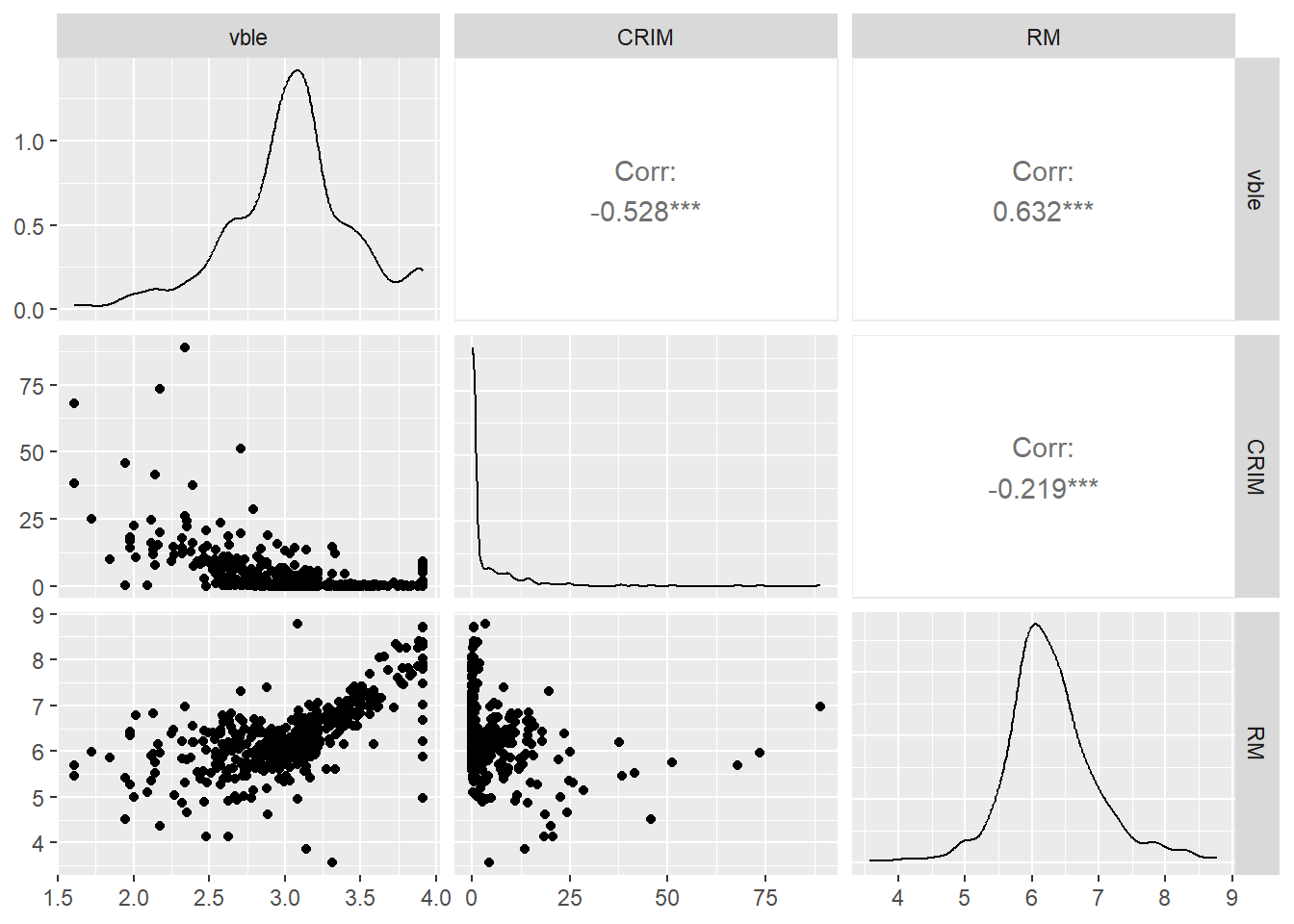
Figure 3.2: Relationship betwen the outcome variable logarithm of housing price (vble), and the covariates per capita crime (CRIM) and number of rooms (RM).
3.2 Model
Let \(Y_i\) be the logarithm of housing price of area \(i\), \(i=1,\ldots,n\). We fit a BYM model that considers \(Y_i\) as the response variable, and crime and number of rooms as covariates:
\[Y_i \sim N(\mu_i, \sigma^2),\ i=1,\ldots,n,\] \[\mu_i = \beta_0 + \beta_1 \times \mbox{crime}_i + \beta_2 \times \mbox{rooms}_i + u_i + v_i.\]
Here, \(\beta_0\) is the intercept, and \(\beta_1\) and \(\beta_2\) represent, respectively, the coefficients of the covariates crime and number of rooms. \(u_i\) is a spatially structured effect modeled with a CAR structure, \(u_i|\mathbf{u_{-i}} \sim N(\bar{u}_{\delta_i}, \frac{\sigma_u^2}{n_{\delta_i}})\). \(v_i\) is an unstructured effect modeled as \(v_i \sim N(0, \sigma_v^2)\).
3.3 Neighbourhood matrix
In the model, the spatial random effect \(u_i\) needs to be specified using a neighborhood structure.
Here, we assume two areas are neighbors if they share a common boundary, and create a neighborhood structure using functions of the spdep package (Bivand 2022).
First, we use the poly2nb() function to create a neighbors list based on areas with contiguous boundaries.
Each element of the list nb represents one area and contains the indices of its neighbors.
For example, nb[[1]] contains the neighbors of area 1.
library(spdep)
library(INLA)
nb <- poly2nb(map)
head(nb)
## [[1]]
## [1] 2 3 6 8 311 313 314 369
##
## [[2]]
## [1] 1 3 4 6
##
## [[3]]
## [1] 1 2 4 5 369 371 375 376
##
## [[4]]
## [1] 2 3 5 6
##
## [[5]]
## [1] 3 4 6 7 375 376 411 413 418
##
## [[6]]
## [1] 1 2 4 5 7 8Then, we use the nb2INLA() function to convert the nb list into a file called map.adj with the representation of the neighborhood matrix as required by R-INLA.
The map.adj file is saved in the working directory which can be obtained with getwd().
Then, we read the map.adj file using the inla.read.graph() function of R-INLA, and store it in the object g which we later use to specify the spatial model using R-INLA.
nb2INLA("map.adj", nb)
g <- inla.read.graph(filename = "map.adj")
3.4 Formula
We specify the model formula by including the response variable, the ~ symbol, and the fixed and random effects. By default, there is an intercept so we do not need to include it in the formula.
In the formula, random effects are specified with the f() function. This function includes as first argument an index vector that specifies the element of the random effect that applies to each observation, and as second argument the model name.
For the spatial random effect \(u_i\), we use model = "besag" with neighborhood matrix given by g.
The option scale.model = TRUE is used to make the precision parameter of models with different CAR priors comparable (Freni-Sterrantino, Ventrucci, and Rue 2018).
For the unstructured effect \(v_i\), we choose model = "iid".
The index vectors of the random effects are given by re_u and re_v created for \(u_i\) and \(v_i\), respectively. These vectors are equal to \(1,\ldots,n\), where \(n\) is the number of areas.
map$re_u <- 1:nrow(map)
map$re_v <- 1:nrow(map)
formula <- vble ~ CRIM + RM +
f(re_u, model = "besag", graph = g, scale.model = TRUE) +
f(re_v, model = "iid")Note that in R-INLA, the BYM model can also be specified with model = "bym" and this comprises both the the spatial and unstructured components. Alternatively, we can use the BYM2 model (Simpson et al. 2017) which is a new parametrization of the BYM model that uses a scaled spatial component \(\boldsymbol{u_*}\) and an unstructured component \(\boldsymbol{v_*}\):
\[\boldsymbol{b} = \frac{1}{\sqrt{\tau_b}}(\sqrt{1-\phi}\boldsymbol{v_*} + \sqrt{\phi}\boldsymbol{u_*}).\]
In this model, the precision parameter \(\tau_b>0\) controls the marginal variance contribution of the weighted sum of \(\boldsymbol{u_*}\) and \(\boldsymbol{v_*}\). The mixing parameter \(0 \leq \phi \leq 1\) measures the proportion of the marginal variance explained by the spatial component \(\boldsymbol{u_*}\). Thus, the BYM2 model is equal to an only spatial model when \(\phi=1\), and an only unstructured spatial noise when \(\phi=0\) (Riebler et al. 2016). The formula of the model using the BYM2 component is specified as follows.
formula <- vble ~ CRIM + RM + f(re_u, model = "bym2", graph = g)3.5 Calling inla()
Then, we fit the model by calling the inla() function specifying the formula, the family, the data, and using the default priors in R-INLA.
We also set control.predictor = list(compute = TRUE) and control.compute = list(return.marginals.predictor = TRUE) to compute and return the posterior means of the predictors.
res <- inla(formula, family = "gaussian", data = map,
control.predictor = list(compute = TRUE),
control.compute = list(return.marginals.predictor = TRUE))
3.6 Results
The resulting object res contains the fit of the model. We can use summary(res) to obtain a summary of the fitted model.
res$summary.fixed contains a summary of the fixed effects.
res$summary.fixedWe observe the intercept \(\hat \beta_0=\) 1.426 with a 95% credible interval equal to (1.253, 1.6). The coefficient of crime is \(\hat \beta_1=\) -0.008 with a 95% credible interval equal to (-0.01, -0.005). This indicates crime is significantly negatively related to housing price. The coefficient of rooms is \(\hat \beta_2=\) 0.26 with a 95% credible interval equal to (0.233, 0.288) indicating number of rooms is significantly positively related to housing price. Thus, the results suggest both crime and number of rooms are important in explaining the spatial pattern of housing prices.
We can type res$summary.fitted.values to obtain a summary of the posterior distributions of the response \(\mu_i\) for each of the areas.
Column mean indicates the posterior mean, and columns 0.025quant and 0.975quant are, respectively, the lower and upper limits of 95% credible intervals representing the uncertainty of the estimates obtained.
summary(res$summary.fitted.values)## mean sd 0.025quant 0.5quant
## Min. :1.610 Min. :0.009630 Min. :1.590 Min. :1.610
## 1st Qu.:2.835 1st Qu.:0.009660 1st Qu.:2.814 1st Qu.:2.835
## Median :3.054 Median :0.009670 Median :3.033 Median :3.054
## Mean :3.035 Mean :0.009683 Mean :3.014 Mean :3.035
## 3rd Qu.:3.219 3rd Qu.:0.009681 3rd Qu.:3.199 3rd Qu.:3.219
## Max. :3.912 Max. :0.011174 Max. :3.892 Max. :3.912
## 0.975quant mode
## Min. :1.632 Min. :1.610
## 1st Qu.:2.856 1st Qu.:2.835
## Median :3.075 Median :3.054
## Mean :3.055 Mean :3.035
## 3rd Qu.:3.240 3rd Qu.:3.219
## Max. :3.933 Max. :3.912We can create variables with the posterior mean (PM) and lower (LL) and upper (UL) limits of 95% credible intervals.
# Posterior mean and 95% CI
map$PM <- res$summary.fitted.values[, "mean"]
map$LL <- res$summary.fitted.values[, "0.025quant"]
map$UL <- res$summary.fitted.values[, "0.975quant"]
Then, we create maps of these variables with mapview specifying a common legend for the three maps, and using a popup table with the name, the logarithm of the housing prices, the covariates, and the posterior mean and 95% credible intervals.
We use the leafsync::sync() function to plot synchronized maps.
# common legend
at <- seq(min(c(map$PM, map$LL, map$UL)),
          max(c(map$PM, map$LL, map$UL)),
          length.out = 8)

# popup table
popuptable <- leafpop::popupTable(dplyr::mutate_if(map, is.numeric,
                                                   round, digits = 2),
zcol = c("TOWN", "vble", "CRIM", "RM", "PM", "LL", "UL"),
row.numbers = FALSE, feature.id = FALSE)

m1 <- mapview(map, zcol = "PM", map.types = "CartoDB.Positron",
              at = at, popup = popuptable)
m2 <- mapview(map, zcol = "LL", map.types = "CartoDB.Positron",
              at = at, popup = popuptable)
m3 <- mapview(map, zcol = "UL", map.types = "CartoDB.Positron",
at = at, popup = popuptable)library(leafsync)
m <- leafsync::sync(m1, m2, m3, ncol = 3)
mWe now obtain estimates of housing prices in their original scale by transforming the estimates of the logarithm of housing prices.
First, we use theinla.tmarginal() function to obtain the marginals of the prices as exp(log(price)).
Then, we use inla.zmarginal() to obtain the summaries of the marginals.
Finally, we create variables PMoriginal, LLoriginal and ULoriginal with the posterior mean and lower and upper limits of 95% credible intervals of the posterior distribution of housing prices.
# Transformation of the marginal of
# the first area with inla.tmarginal()
# inla.tmarginal(function(x) exp(x),
#                res$marginals.fitted.values[[1]])

# Transformation marginals with inla.tmarginal()
marginals <- lapply(res$marginals.fitted.values,
FUN = function(marg){inla.tmarginal(function(x) exp(x), marg)})

# Obtain summaries of the marginals with inla.zmarginal()
marginals_summaries <- lapply(marginals,
FUN = function(marg){inla.zmarginal(marg)})

# Posterior mean and 95% CI
map$PMoriginal <- sapply(marginals_summaries, '[[', "mean")
map$LLoriginal <- sapply(marginals_summaries, '[[', "quant0.025")
map$ULoriginal <- sapply(marginals_summaries, '[[', "quant0.975")
We create maps with the estimated prices and lower and upper 95% credible intervals. The inspection of these maps allows us to understand the spatial pattern of housing prices in Boston, as well as the uncertainty in the estimates.
# common legend
at <- seq(min(c(map$PMoriginal, map$LLoriginal, map$ULoriginal)),
          max(c(map$PMoriginal, map$LLoriginal, map$ULoriginal)),
          length.out = 8)

# popup table
popuptable <- leafpop::popupTable(dplyr::mutate_if(map, is.numeric,
                                                   round, digits = 2),
zcol = c("TOWN", "vble", "CRIM", "RM", "PM", "LL", "UL"),
row.numbers = FALSE, feature.id = FALSE)

m1 <- mapview(map, zcol = "PMoriginal",
              map.types = "CartoDB.Positron",
              at = at, popup = popuptable)
m2 <- mapview(map, zcol = "LLoriginal",
              map.types = "CartoDB.Positron",
              at = at, popup = popuptable)
m3 <- mapview(map, zcol = "ULoriginal",
              map.types = "CartoDB.Positron",
              at = at, popup = popuptable)
m <- leafsync::sync(m1, m2, m3, ncol = 3)
m