Spatial autocorrelation

Paula Moraga, KAUST

Materials based on the book Geospatial Health Data (2019, Chapman & Hall/CRC)
http://www.paulamoraga.com/book-geospatial

1 Spatial autocorrelation

Spatial autocorrelation is used to describe the extent to which a variable is correlated with itself through space. This concept is closely related to Tobler’s First Law of Geography, which states that “everything is related to everything else, but near things are more related than distant things” (Tobler 1970). Positive spatial autocorrelation occurs when observations with similar values are closer together (i.e. clustered). Negative spatial autocorrelation occurs when observations with dissimilar values are closer together (i.e. dispersed). Figure 1.1 shows three configurations of areas showing different types of spatial autocorrelation.

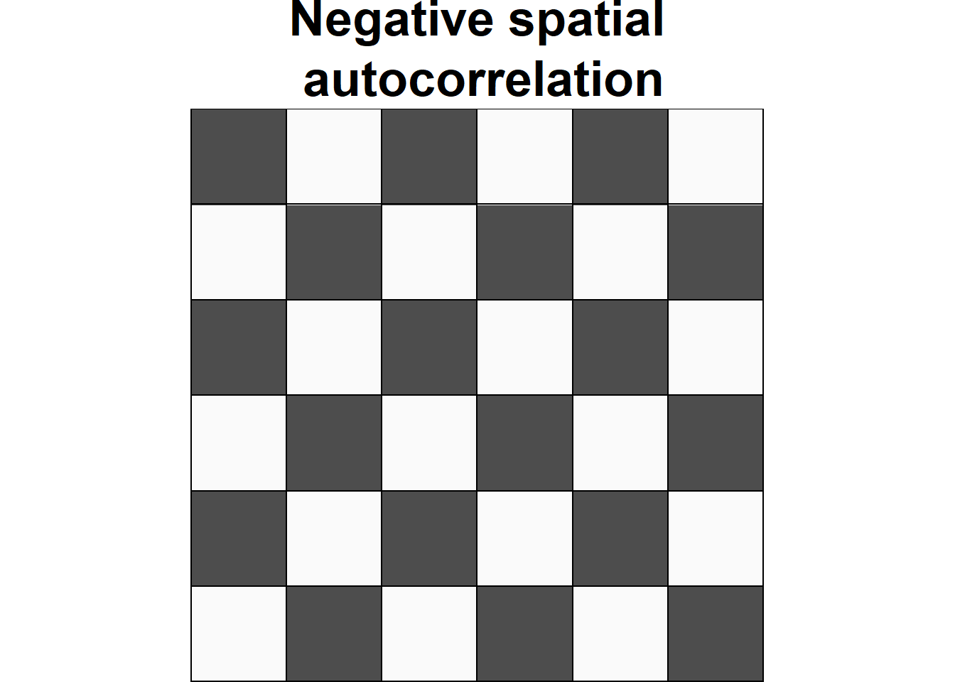
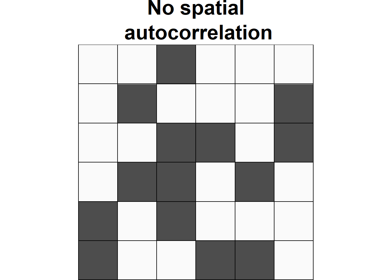
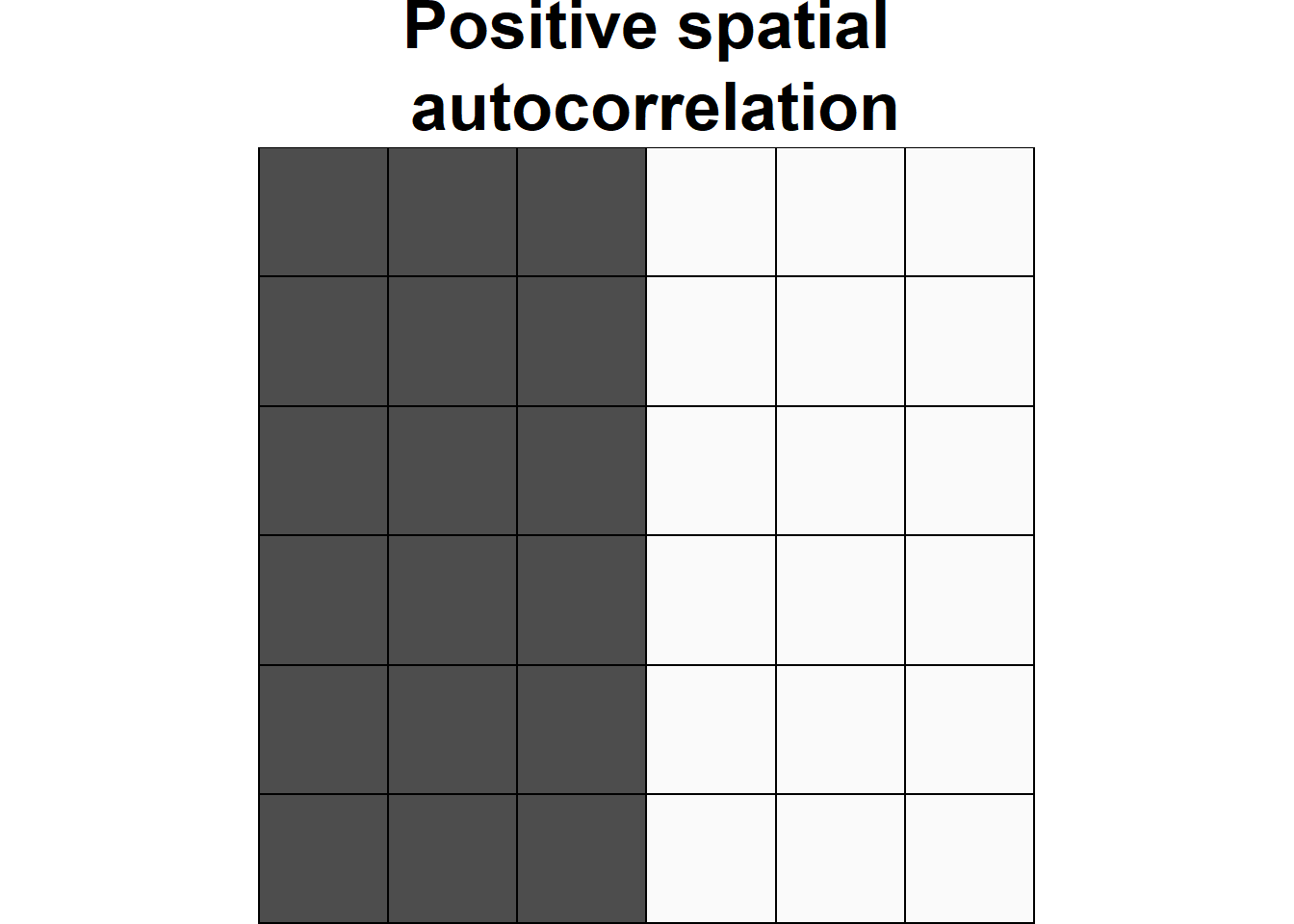
Figure 1.1: Examples of configurations of areas showing different types of spatial autocorrelation.

Spatial autocorrelation can be assessed using indices that summarize the degree to which similar observations tend to occur near each other over the study area. Two common indices that are used to assess spatial autocorrelation in areal data are Moran’s \(I\) (Moran 1950) and Geary’s \(C\) (Geary 1954).

In this chapter, we use the Moran’s \(I\) to test the spatial autocorrelation of housing prices in Boston, USA. Specifically, we use the boston data from the spData package (Bivand, Nowosad, and Lovelace 2022) that contains housing data corresponding to 506 Boston census tracts in 1978. The boston data has a variable called MEDV with the median prices of owner-occupied housing in USD 1000. We create the variable vble with the values of MEDV that will be used in the analysis. Figure 1.2 shows the map created with the housing prices using mapview (Appelhans et al. 2022).

library(spData)
library(sf)
library(mapview)
map <- st_read(system.file("shapes/boston_tracts.shp",
                           package = "spData"), quiet = TRUE)
map$vble <- map$MED
mapview(map, zcol = "vble")

Figure 1.2: Median prices of owner-occupied housing in USD 1000 in cencus tracts of Boston in 1978.

2 Global Moran’s \(I\)

Th Global Moran’s \(I\) (Moran 1950) takes the form

\[I = \frac{n \sum_i \sum_j w_{ij}(Y_i - \bar Y)(Y_j - \bar Y)} {(\sum_{i \neq j} w_{ij}) \sum_i (Y_i - \bar Y)^2},\]

where \(n\) is the number of regions, \(Y_i\) is the observed value of the variable of interest in region \(i\), and \(\bar Y\) is the mean of all values. \(w_{ij}\) are spatial weights that denote the spatial proximity between regions \(i\) and \(j\), with \(w_{ii} = 0\) and \(i, j=1,\ldots,n\). The definition of the spatial weights depends on the variable of study and the specific setting.

We can test the presence of spatial autocorrelation using the Moran’s \(I\), which quantifies how similar each region is with its neighbors and averages all these assessments. Under the null hypothesis of no spatial autocorrelation, observations \(Y_i\) are independent identically distributed, and \(I\) is asymptotically normally distributed with mean and variance equal to \[E[I] = \frac{-1}{n-1}\] and \[Var[I] = \frac{n^2(n-1)S_1 - n(n-1)S_2 - 2 S_0^2}{(n+1)(n-1)^2 S_0^2},\] where \[S_0 = \sum_{i \neq j} w_{ij},\ S_1= \frac{1}{2}\sum_{i\neq j} (w_{ij}+w_{ji})^2,\mbox{ and } S_2 = \sum_k \left(\sum_j w_{kj}+\sum_i w_{ik}\right)^2.\]

Moran’s \(I\) values usually range from -1 to 1. Moran’s \(I\) values significantly above \(E[I] = -1/(n-1)\) indicate positive spatial autocorrelation or clustering. This occurs when neighboring regions tend to have similar values. Moran’s \(I\) values significantly below \(E[I]\) indicate negative spatial autocorrelation or dispersion. This happens when regions that are close to one another tend to have different values. Finally, Moran’s \(I\) values around \(E[I]\) indicate randomness, that is, absence of spatial pattern.

When the number of regions is sufficiently large, \(I\) has a normal distribution and we can assess whether any given pattern deviates significantly from a random pattern by comparing the z-score

\[z = \frac{I-E(I)}{Var(I)^{1/2}}\]

to the standard normal distribution. An alternative approach to judge significance is Monte Carlo randomization. This method creates random patterns by reassigning the observed values among the areas and calculates the Moran’s \(I\) for each of the patterns, providing a randomization distribution for the Moran’s \(I\). If the observed value of Moran’s \(I\) lies in the tails of this distribution, the assumption of independence among observations is rejected. Thus, we can test spatial autocorrelation by following these steps:

1. State the null and alternative hypotheses:
   \(H_0: I = E[I]\) (no spatial autocorrelation),
   \(H_1: I \neq E[I]\) (spatial autocorrelation).

2. Choose the significance level \(\alpha\) which represents the maximum value for the probability of incorrectly rejecting the null hypothesis when it is true we are willing to tolerate (usually \(\alpha = 0.05\)).

3. Calculate the test statistic: \[z = \frac{I-E(I)}{Var(I)^{1/2}}.\]

4. Find the p-value for the observed data by comparing the z-score to the standard normal distribution or via Monte Carlo randomization. The p-value is the probability of obtaining a test statistic as extreme as or more extreme than the one observed test statistic in the direction of the alternative hypothesis, assuming the null hypothesis is true.

5. Make one of these two decisions and state a conclusion.
   If p-value \(< \alpha\), we reject the null hypothesis. We conclude data provide evidence for the alternative hypothesis.
   If p-value \(\geq \alpha\), we fail to reject the null hypothesis. The data do not provide evidence for the alternative hypothesis.

3 The moran.test() function

The function moran.test() of the spdep package can be used to test spatial autocorrelation using Moran’s \(I\). The arguments of moran.test() are a numeric vector with the data, a list with the spatial weights, and the type of hypothesis. The argument that denotes the hypothesis is called alternative and can be set equal to greater (default), less or two.sided to represent different alternative hypothesis. In this example, we specify the null and alternative hypothesis as follows,

\(H_0: I \leq E[I]\) (negative spatial autocorrelation or no spatial autocorrelation),
\(H_1: I > E[I]\) (positive spatial autocorrelation).

We use moran.test() to test this hypothesis by setting alternative = "greater". The list with the spatial weights is calculated by first obtaining the neighbors of each area with the poly2nb() function, and then creating a list containing the neighbors with the nb2listw() function of spdep.

# Neighbors
library(spdep)
nb <- poly2nb(map, queen = TRUE) # queen shares point or border
nbw <- nb2listw(nb, style = "W")

# Global Moran's I
gmoran <- moran.test(map$vble, nbw,
                     alternative = "greater")
gmoran

## 
##  Moran I test under randomisation
## 
## data:  map$vble  
## weights: nbw    
## 
## Moran I statistic standard deviate = 23.35, p-value < 2.2e-16
## alternative hypothesis: greater
## sample estimates:
## Moran I statistic       Expectation          Variance 
##      0.6266753872     -0.0019801980      0.0007248686

gmoran[["estimate"]][["Moran I statistic"]] # Moran's I

## [1] 0.6266754

gmoran[["statistic"]] # z-score

## Moran I statistic standard deviate 
##                            23.3498

gmoran[["p.value"]] # p-value

## [1] 6.923334e-121

The object returned by moran.test() provides the Moran’s \(I\) statistic, the z-score and the p-value. We observe the p-value obtained is lower than the significance level 0.05. Then, we reject the null hypothesis and conclude there is evidence for positive spatial autocorrelation.

The same conclusion is obtained if we use a Monte Carlo approach to assess significance. This approach creates random patterns by reassigning the values among the fixed areas and calculates the Moran’s \(I\) for each of these patterns. Then, it calculates the p-value as the proportion of values as extreme or more extreme than the statistic observed in the direction of the alternative hypothesis. Here, we conduct a Monte Carlo randomization approach using the moran.mc() function setting the number of simulations to nsim = 999. Figure 3.1 shows the histogram of the Moran’s \(I\) values for each of the simulated patterns, as well as the Moran’s \(I\) obtained with the real data. We observe a p-value lower than 0.05 indicating that the data presents positive spatial autocorrelation.

gmoranMC <- moran.mc(map$vble, nbw, nsim = 999)
gmoranMC

## 
##  Monte-Carlo simulation of Moran I
## 
## data:  map$vble 
## weights: nbw  
## number of simulations + 1: 1000 
## 
## statistic = 0.62668, observed rank = 1000, p-value = 0.001
## alternative hypothesis: greater

hist(gmoranMC$res)
abline(v = gmoranMC$statistic, col = "red")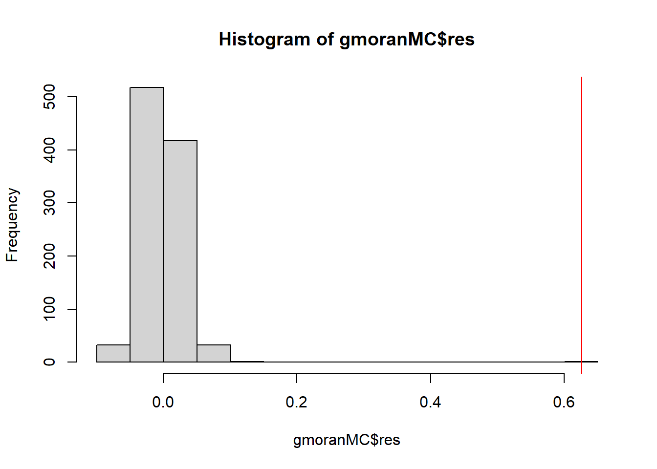

Figure 3.1: Histogram of the Moran’s \(I\) values for each of the simulated patterns in the Monte Carlo randomization approach. The red line represents the Moran’s \(I\) obtained for the real data.

4 Moran’s \(I\) scatterplot

The moran.plot() function can be used to construct a Moran’s \(I\) scatterplot to visualize the spatial autocorrelation in the data. This plot displays the observations of each area against its spatially lagged values. The spatially lagged value for a given area is calculated as a weighted average of the neighboring values for that area. This value can be computed, for example, using the lag.listw() function of spdep passing the values and the spatial weights corresponding to the areas. Figure 4.1 shows the Moran’s \(I\) scatterplot for the housing prices data obtained with the moran.plot() function passing the housing prices and the spatial weights corresponding to the Boston tracts. We observe a positive linear relationship between the observations and their spatially lagged values. Using this plot, we can also identify data points that have a high influence on the linear relationship between the data and the lagged values.

moran.plot(map$vble, nbw)

Figure 4.1: Moran’s \(I\) scatterplot showing the observations against its spatially lagged values.

5 Local Moran’s \(I\)

We have seen that the Global Moran’s \(I\) provides an index to assess the spatial autocorrelation for the whole study region. There is often interest in providing a local measure of similarity between each area’s value and those of nearby areas. Local Indicators of Spatial Association (LISA) (Anselin 1995) are designed to provide an indication of the extent of significant spatial clustering of similar values around each observation. A desirable property is that the sum of the LISA’s values across all regions is equal to a multiple of the global indicator of spatial association. As a result, global statistics may be decomposed into a set of local statistics and most LISAs are defined as local versions of well-known global indexes.

One of the most popular LISAs is the local version of Moran’s \(I\). For the \(i\)th region, the local Moran’s \(I\) defined as

\[I_i = \frac{n (Y_i - \bar Y)}{\sum_j (Y_j - \bar Y)^2} \sum_j w_{ij}(Y_j - \bar Y).\]

Note that the global Moran’s \(I\) is proportional to the sum of the local Moran’s \(I\) obtained for all regions:

\[I = \frac{1}{\sum_{i \neq j} w_{ij}}\sum_i I_i.\]

Typically, the values of the LISAs are mapped to indicate the location of areas with comparatively high or low local association with neighboring areas. A high value for \(I_i\) suggests that the area is surrounded by areas with similar values. Such an area is part of a cluster of high observations, low observations, or moderate observations. A low value for \(I_i\) indicates that the area is surrounded by areas with dissimilar values. Such an area is an outlier indicating that the observation of area \(i\) is different from most or all of the observations of its neighbors.

To interpret the local Moran’s \(I\) for each of the areas, it is necessary to compute a map of p-values representing the probability of exceeding the observed values assuming the null hypothesis is true. These p-values, regardless of the presence or absence of global spatial association, may be obtained by a simulation process with a conditional randomization approach. In this approach, the observed value \(Y_i\) at region \(i\) is fixed, and the remaining values are randomly reassigned over the other regions.

6 The localmoran() function

The localmoran() function of the spdep package can be used to compute the Local Moran’s \(I\) for a given dataset. The arguments of localmoran() include a numeric vector with the values of the variable, a list with the neighbor weights, and the name of alternative hypothesis that can be set equal to greater (default), less or two.sided. The returned object of the localmoran() function contains the following information:

• Ii: Local Moran’ \(I\) statistic for each area,
• E.Ii: Expectation Local Moran’ \(I\) statistic,
• Var.Ii: Variance Local Moran’ \(I\) statistic,
• Z.Ii: z-score,
• Pr(z > E(Ii)), Pr(z < E(Ii)) or Pr(z != E(Ii)): p-value for alternative hypothesis greater, less or two.sided, respectively.

Here, we use the localmoran() function to compute the Local Moran’s \(I\) for the housing prices data. We set alternative = "greater" which corresponds to testing \(H_0\): no or negative spatial autocorrelation vs. \(H_1\): positive spatial autocorrelation.

lmoran <- localmoran(map$vble, nbw, alternative = "greater")
head(lmoran)

##              Ii          E.Ii       Var.Ii        Z.Ii Pr(z > E(Ii))
## 1 -0.3457508492 -5.254157e-04 3.275376e-02 -1.90753363  9.717742e-01
## 2  0.0175875407 -1.626873e-05 2.045711e-03  0.38921049  3.485602e-01
## 3  0.0123379633 -6.557001e-07 4.089699e-05  1.92939381  2.684100e-02
## 4 -0.0001654033 -1.059064e-07 1.331742e-05 -0.04529559  5.180641e-01
## 5  0.3591628595 -1.427815e-04 7.898947e-03  4.04277384  2.641128e-05
## 6  0.0545610965 -1.625936e-04 1.357382e-02  0.46970410  3.192832e-01

We create maps with tmap (Tennekes 2022) showing the housing prices, the local Moran’s \(I\), z-scores and p-values. Areas with p-value less than the significance level 0.05 (or with z-scores higher than qnorm(0.95) = 1.65) correspond to areas for which we would reject the null hypothesis and conclude they present positive spatial autocorrelation.

library(tmap)
tmap_mode("view")

map$lmI <- lmoran[, "Ii"] # local Moran's I
map$lmZ <- lmoran[, "Z.Ii"] # z-scores
# p-values corresponding to alternative greater
map$lmp <- lmoran[, "Pr(z > E(Ii))"]

p1 <- tm_shape(map) +
  tm_polygons(col = "vble", title = "vble", style = "quantile") +
  tm_layout(legend.outside = TRUE)

p2 <- tm_shape(map) +
  tm_polygons(col = "lmI", title = "Local Moran's I", style = "quantile") +
  tm_layout(legend.outside = TRUE)

p3 <- tm_shape(map) +
  tm_polygons(col = "lmZ", title = "Z-score", breaks = c(-Inf, 1.65, Inf)) +
  tm_layout(legend.outside = TRUE)

p4 <- tm_shape(map) +
  tm_polygons(col = "lmp", title = "p-value", breaks = c(-Inf, 0.05, Inf)) +
  tm_layout(legend.outside = TRUE)

tmap_arrange(p1, p2, p3, p4)

If we used alternative = "two.sided" instead of alternative = "greater", we would be testing \(H_0\): no spatial autocorrelation vs. \(H_1\): positive or negative spatial autocorrelation. In this two-sided test, z-score values lower than -1.96 indicate negative spatial autocorrelation, and z-score values greater than 1.96 indicate positive spatial autocorrelation. The map below shows the areas with negative, no, and positive spatial autocorrelation, obtained by breaking the legend according to these z-score values.

tm_shape(map) + tm_polygons(col = "lmZ",
title = "Local Moran's I", style = "fixed",
breaks = c(-Inf, -1.96, 1.96, Inf),
labels = c("Negative SAC", "No SAC", "Positive SAC"),
palette =  c("blue", "white", "red")) +
tm_layout(legend.outside = TRUE)

7 Clusters

Local Moran’s \(I\) allows us to identify clusters of the following types:

• High-High: areas of high values with neighbors of high values,
• High-Low: areas of high values with neighbors of low values,
• Low-High: areas of low values with neighbors of high values,
• Low-Low: areas of low values with neighbors of low values.

To detect clusters, we first use the localmoran() function to calculate the local Moran’s \(I\). The p-values for the alternative hypothesis "two.sided" are in column 5 of the returned object.

lmoran <- localmoran(map$vble, nbw, alternative = "two.sided")
head(lmoran)

##              Ii          E.Ii       Var.Ii        Z.Ii Pr(z != E(Ii))
## 1 -0.3457508492 -5.254157e-04 3.275376e-02 -1.90753363   5.645152e-02
## 2  0.0175875407 -1.626873e-05 2.045711e-03  0.38921049   6.971204e-01
## 3  0.0123379633 -6.557001e-07 4.089699e-05  1.92939381   5.368199e-02
## 4 -0.0001654033 -1.059064e-07 1.331742e-05 -0.04529559   9.638717e-01
## 5  0.3591628595 -1.427815e-04 7.898947e-03  4.04277384   5.282257e-05
## 6  0.0545610965 -1.625936e-04 1.357382e-02  0.46970410   6.385664e-01

map$lmp <- lmoran[, 5] # p-values are in column 5

Then, we identify the clusters of each type by using the information provided by the Moran’s \(I\) scatterplot obtained with the moran.plot() function (Figure 7.1).

mp <- moran.plot(as.vector(scale(map$vble)), nbw)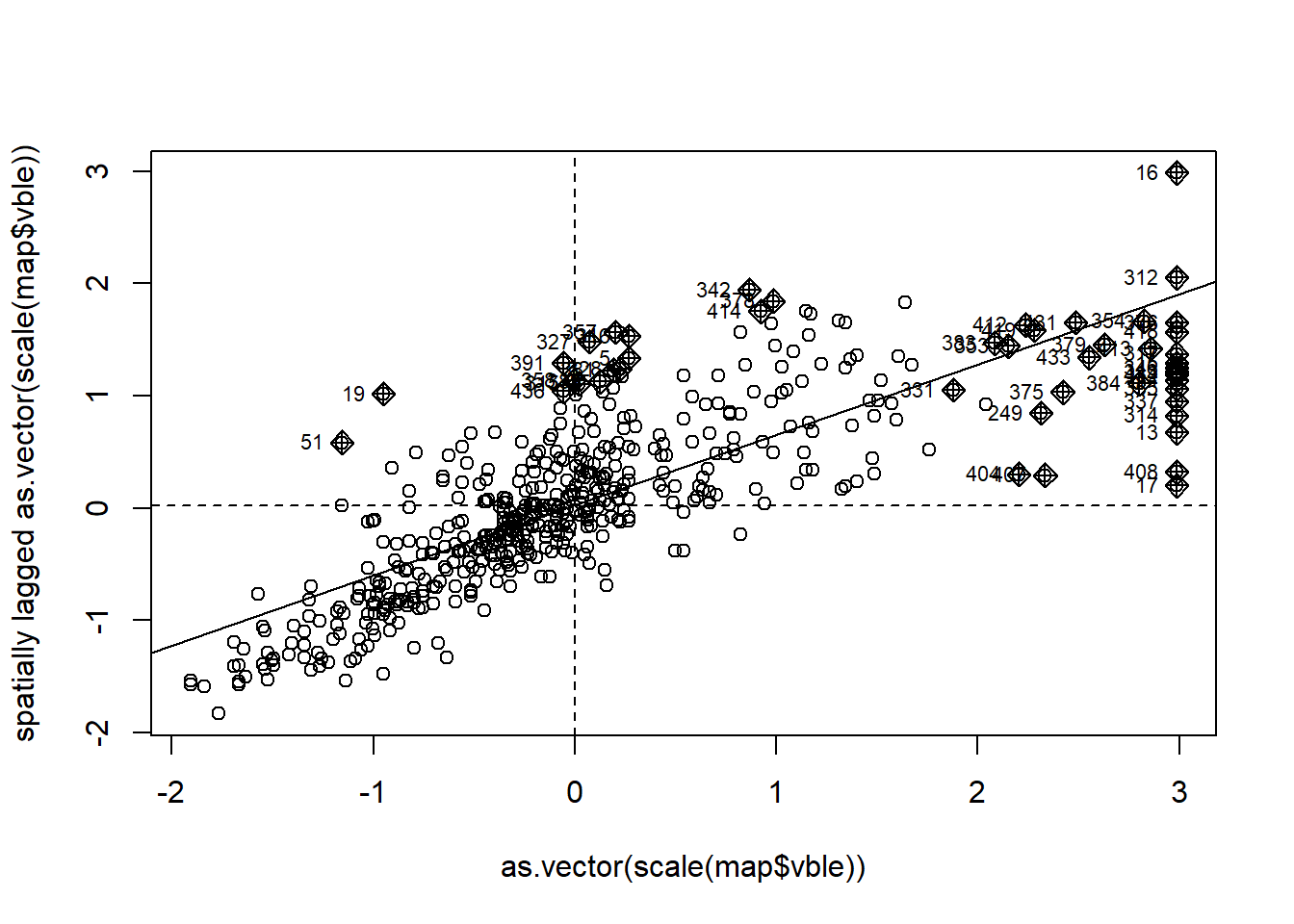

Figure 7.1: Moran’s \(I\) scatterplot showing the scaled values against its spatially lagged values.

head(mp)

Specifically, we identify the cluster types by using the quadrants of the scaled values (mp$x) and their spatially lagged values (mp$wx), and the p-values obtained with the local Moran’s \(I\) for each of the areas (map$lmp). The classification of the clusters is as follows. Areas with significant local Moran’s \(I\) are classified as high-high if both the value and its corresponding spatially lagged value are positive, low-low if both the value and its spatially lagged value are negative, high-low if the the value is positive and the spatially lagged value negative, and low-high is the value is negative and the spatially lagged value positive.

We create the variable quadrant denoting the type of cluster for each of the areas using the quadrant corresponding to its value and its spatially lagged value, and the p-value. Specifically, areas with quadrant equal to 1, 2, 3, and 4 correspond to clusters of type high-high, low-low, high-low, and low-high, respectively. Areas with quadrant equal to 5 are non-significant.

map$quadrant <- NA
map[(mp$x >= 0 & mp$wx >= 0) & (map$lmp <= 0.05), "quadrant"] <- 1 # high-high
map[(mp$x <= 0 & mp$wx <= 0) & (map$lmp <= 0.05), "quadrant"] <- 2 # low-low
map[(mp$x >= 0 & mp$wx <= 0) & (map$lmp <= 0.05), "quadrant"] <- 3 # high-low
map[(mp$x <= 0 & mp$wx >= 0) & (map$lmp <= 0.05), "quadrant"] <- 4 # low-high
map[(map$lmp > 0.05), "quadrant"] <- 5 # non-significant

The map below shows the clusters obtained with the Boston housing prices data.

tm_shape(map) + tm_fill(col = "quadrant", title = "",
breaks = c(1, 2, 3, 4, 5, 6),
palette =  c("red", "blue", "lightpink", "skyblue2", "white"),
labels = c("High-High", "Low-Low", "High-Low",
           "Low-High", "Not significant")) +
tm_legend(text.size = 1)  + tm_borders(alpha = 0.5) +
tm_layout(frame = FALSE,  title = "Clusters")  +
tm_layout(legend.outside = TRUE)

References

Anselin, Luc. 1995. “Local Indicators of Spatial Association - LISA.” Geographical Analysis 27: 93–115. https://doi.org/https://doi.org/10.1111/j.1538-4632.1995.tb00338.x.

Appelhans, Tim, Florian Detsch, Christoph Reudenbach, and Stefan Woellauer. 2022. Mapview: Interactive Viewing of Spatial Data in r. https://github.com/r-spatial/mapview.

Bivand, Roger, Jakub Nowosad, and Robin Lovelace. 2022. spData: Datasets for Spatial Analysis. https://jakubnowosad.com/spData/.

Geary, R. C. 1954. “The Contiguity Ratio and Statistical Mapping.” The Incorporated Statistician 5 (3): 115–46. https://doi.org/https://doi.org/10.2307/2986645.

Moran, P. A. P. 1950. “Notes on Continuous Stochastic Phenomena.” Biometrika 37 (1/2): 17–23. https://doi.org/https://doi.org/10.2307/2332142.

Tennekes, Martijn. 2022. Tmap: Thematic Maps. https://github.com/r-tmap/tmap.

Tobler, W. R. 1970. “A Computer Movie Simulating Urban Growth in the Detroit Region.” Economic Geography 46: 234–40. https://doi.org/https://doi.org/10.2307/143141.