Spatial neighborhood matrices

Paula Moraga, KAUST

Materials based on the book Geospatial Health Data (2019, Chapman & Hall/CRC)
http://www.paulamoraga.com/book-geospatial

Areal or lattice data arise when a study region is partitioned into a finite number of areas at which outcomes are aggregated. Examples of areal data are the number of individuals with a certain disease in municipalities of a country, the number of road accidents in provinces, or the average housing prices in districts of a city.

The concept of spatial neighborhood is useful for the exploration of areal data to assess spatial autocorrelation and find out whether close areas have similar or dissimilar values. Spatial neighbors can be defined in several ways depending on the variable of interest and the specific setting. The simplest neighborhood definition assumes that neighbors are areas that share a common border, perhaps a vertex. We can also expand the idea of neighborhood to include areas that are close, but not necessarily adjacent, by assuming neighbors are areas that are within some distance apart.

Given a spatial neighborhood definition, we can construct a spatial neighborhood matrix which will allow us to assess spatial autocorrelation. The elements of the spatial neighborhood matrix can be viewed as weights that spatially connect areas. In this matrix, entries corresponding to close areas will have more weight than entries corresponding to areas that are farther apart.

The spdep package (Bivand 2022) contains a number of functions to deal with spatial dependence structures. Some of its functions can be used to construct spatial neighborhood matrices and perform spatial autocorrelation analyses. For example, the functions poly2nb() and dnearneigh() can be used to create neighbor lists based on contiguity and distance criteria, respectively. Spatial neighborhood matrices can be built from the neighbor lists using the nb2listw() function.

In this chapter, we demonstrate how to use the spdep package to construct several types of spatial neighborhood structures and matrices using the map of the 49 neighborhoods of Columbus, USA. We read the map which is in the columbus shapefile of the spData package and assign it to a variable called map as follows.

library(spData)
library(sf)
library(spdep)
library(ggplot2)
map <- st_read(system.file("shapes/columbus.shp",
               package = "spData"), quiet = TRUE)

1 Neighbors based on contiguity

Neighbors based on contiguity are constructed by assuming that neighbors of a given area are other areas that share a common boundary. Figure 1.1 shows two types of contiguity neighbors. Neighbors can be of type Queen if a single shared boundary point meets the contiguity condition, or Rook if more than one shared point is required to meet the contiguity condition.

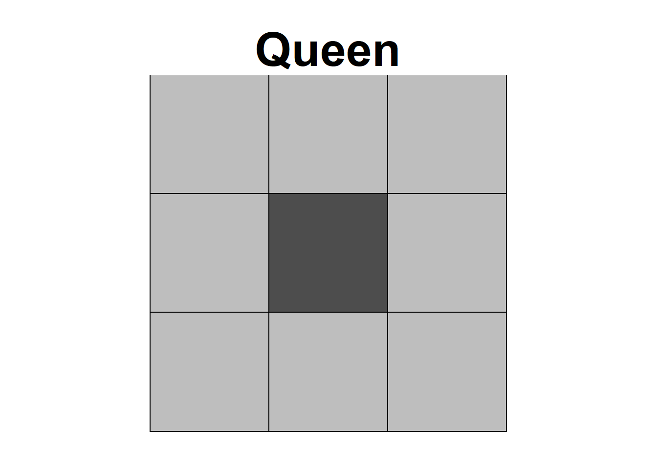
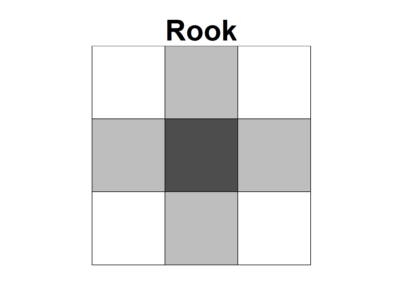
Figure 1.1: Neighbors based on contiguity. Area of interest is represented in black and its neighbors in gray.

The function poly2nb() of the spdep package can be used to construct a list of neighbors based on areas with contiguous boundaries, that is, areas sharing one or more boundary point. poly2nb() accepts a list of polygons and returns a list of class nb with the neighbors of each area. The default type in poly2nb() is queen = TRUE so neighbors of a given area are other areas sharing a common point or more than one point. Here, we use poly2nb() to calculate the neighbors of each of the regions of Columbus based on Queen contiguity.

library(spdep)
nb <- spdep::poly2nb(map, queen = TRUE)
head(nb)

## [[1]]
## [1] 2 3
## 
## [[2]]
## [1] 1 3 4
## 
## [[3]]
## [1] 1 2 4 5
## 
## [[4]]
## [1] 2 3 5 8
## 
## [[5]]
## [1]  3  4  6  8  9 11 15 16
## 
## [[6]]
## [1] 5 9

Figure 1.2 shows a map with the neighbors obtained. This plot is obtained by first plotting the map, and then overlapping the neighborhood structure with the plot.nb() function passing the neighbor list and the coordinates of the map.

plot(st_geometry(map), border = "lightgrey")
plot.nb(nb, st_geometry(map), add = TRUE)

We can plot the neighbors of a given area by adding a new column in map representing the neighbors of the area. For example, Figure 1.2 shows the neighbors of area 20.

id <- 20 # area id
map$neighbors <- "other"
map$neighbors[id] <- "area"
map$neighbors[nb[[id]]] <- "neighbors"
ggplot(map) + geom_sf(aes(fill = neighbors)) +
  theme_bw() + scale_fill_manual(values = c("gray30", "gray", "white"))

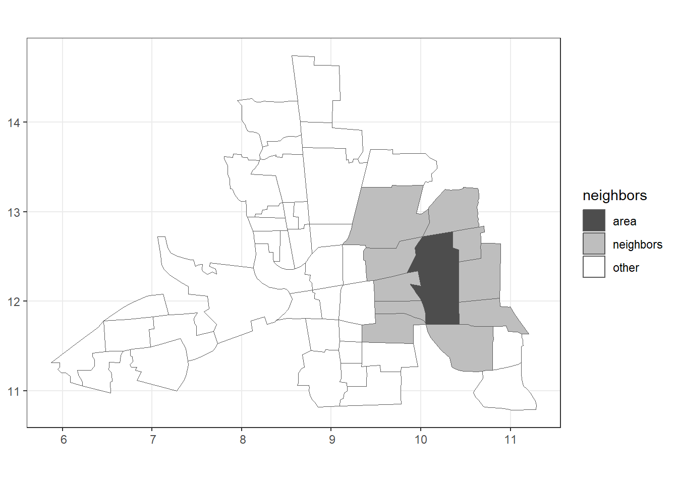
Figure 1.2: Left: Map of neighbors based on contiguity. Right: Map of neighbors of area 20 based on contiguity.

Given a neighbor list, the cardinality function spdep::card() counts the number of neighbors of each area. We can also obtain the number of neighbors of each area with lengths(nb). Then, we can use table(1:nrow(map), card(nb)) to build a table with the areas’ ids in rows, and the number of neighbors in columns.

2 Neighbors based on \(k\) nearest neighbors

We can also consider as neighbors of an area its \(k\) nearest neighbors based on the distance separating them. For example, Figure 2.1 represents the 3 nearest neighbors of an area. The function knearneigh() of spdep allows us to obtain a matrix with the indices of points belonging to the set of the \(k\) nearest neighbors of each area. The arguments of this function include a matrix of point coordinates and the number k of nearest neighbors to be returned. Then, we can use knn2nb() to convert this list into a neighbor list of class nb with the integer vectors containing the ids of the neighbors. Figure 2.1 shows a map of the nearest neighbors of map with order \(k=3\).

# Neighbors based on 3 nearest neighbors
coo <- st_centroid(map)
nb <- knn2nb(knearneigh(coo, k = 3)) # k number nearest neighbors
head(nb)
plot(st_geometry(map), border = "lightgrey")
plot.nb(nb, st_geometry(map), add = TRUE)

## [[1]]
## [1] 2 3 4
## 
## [[2]]
## [1] 1 4 8
## 
## [[3]]
## [1] 1 4 5
## 
## [[4]]
## [1] 2 7 8
## 
## [[5]]
## [1]  3  8 11
## 
## [[6]]
## [1]  5  9 10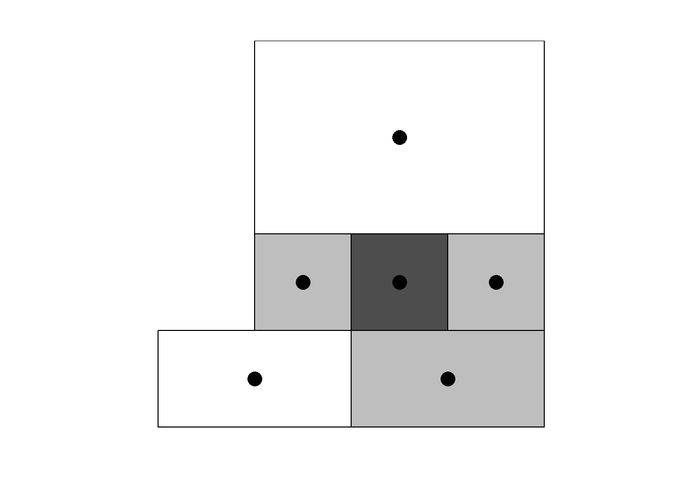

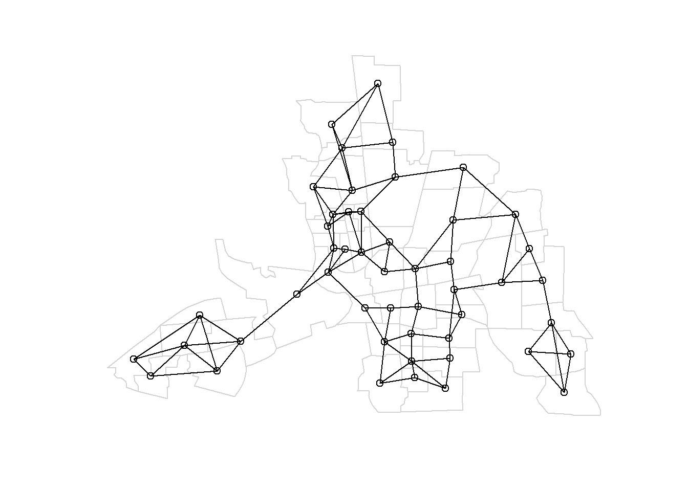
Figure 2.1: Left: Neighbors based on 3 nearest neighbors. Area of interest is represented in black and its neighbors in gray. Right: Map of neighbors based on 3 nearest neighbors.

3 Neighbors based on distance

Neigborhood structures can also be defined by considering neighbors areas that are within a given distance (Figure 3.1). The dnearneigh() function of spdep builds a list of neighbors based on a distance between specific lower and upper bounds. The arguments of dnearneigh() include the object with the point coordinates, and the lower and upper distance bounds (d1 and d2). For example, Figure 3.1 shows the map of neighbors obtained by considering neighbors areas separated by a distance less than 0.4.

# Neighbors based on distance
nb <- dnearneigh(x = st_centroid(map), d1 = 0, d2 = 0.4)
head(nb)
plot(st_geometry(map), border = "lightgrey")
plot.nb(nb, st_geometry(map), add = TRUE)

## [[1]]
## [1] 0
## 
## [[2]]
## [1] 4
## 
## [[3]]
## [1] 0
## 
## [[4]]
## [1] 2 8
## 
## [[5]]
## [1] 0
## 
## [[6]]
## [1] 0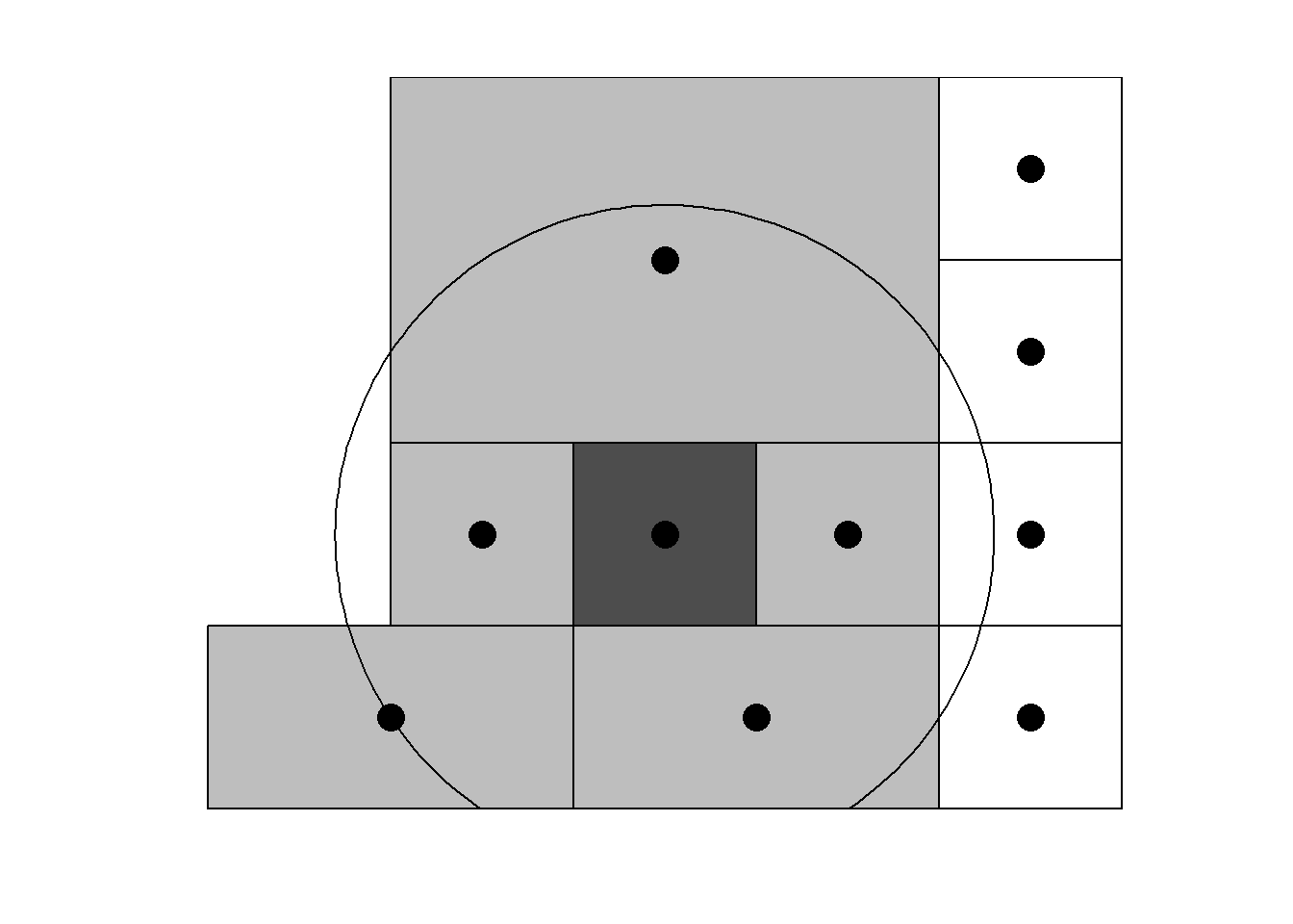

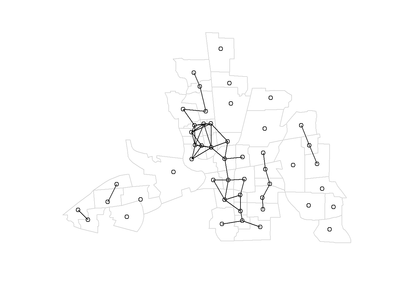
Figure 3.1: Left: Neighbors based on distance. Area of interest is represented in black and its neighbors in gray. Circle’s center is the centroid of the area of interest, and circle’s radius is the distance. Right: Map of neighbors separated by a distance less than 0.4.

Note that we can also determine an appropriate upper distance to ensure that each area has at least k neighbors. To determine an appropriate upper distance bound for a given number of neighbors k preferred, we can proceed as follows. First, we use the spdep::knearneigh() function to obtain the k nearest neighbors of each of the areas. We use this function passing a matrix of point coordinates and the number k of chosen nearest neighbors to obtain a matrix with the k nearest neighbors of each area. Then, we use spdep::knn2nb() to convert this list into a neighbor list of class nb with the ids of the neighbors. For example, here we determine the upper distance bound to ensure all areas have at least one neighbor.

coo <- st_centroid(map)
nb1 <- knn2nb(knearneigh(coo, k = 1)) # k is the number nearest neighbors
# head(nb1)

Then, we use spdep::nbdists() passing the nb list with the neighbors and the matrix of point coordinates to obtain the distances along the links. Finally, we can compute summaries to determine the upper distance bound.

dist1 <- nbdists(nb1, coo)
# head(dist1)
summary(unlist(dist1))

##    Min. 1st Qu.  Median    Mean 3rd Qu.    Max. 
##  0.1276  0.2543  0.3164  0.3291  0.4044  0.6189

In this example, the maximum distance is 0.62 and we can take this value as an upper bound of the distance to ensure each area has at least one neighbor.

4 Neighbors of order \(k\) based on contiguity

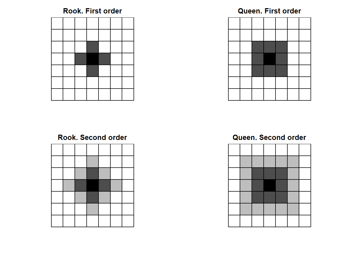
Figure 4.1: Rook and Queen neighbors of first (dark gray) and second (light gray) order.

Figure 4.1 shows first and second order neighbors based on contiguity. The nblab() function of the spdep package creates higher order neighbor lists, where higher order neighbors are lags links from each other on the graph described by the input neighbors list of class nb. The arguments of this function are a neighbors list of class nb, and the maximum lag considered. The returned object is a list of lagged neighbors lists each with class nb.

Here, we use nblag() with the maximum lag equal to maxlag = 2 to create a list containing a list of neighbors of order 1, and a list of neighbors of order 2 (Figure 4.2).

library(spdep)
nb <- poly2nb(map, queen = TRUE)
nblags <- spdep::nblag(neighbours = nb, maxlag = 2)

# Neighbors of first order
plot(st_geometry(map), border = "lightgrey")
plot.nb(nblags[[1]], st_geometry(map), add = TRUE)

# Neighbors of second order
plot(st_geometry(map), border = "lightgrey")
plot.nb(nblags[[2]], st_geometry(map), add = TRUE)

The function nblag_cumul() of spdep cumulates a list of lagged neighbors as the output of nblag() and returns a single neighbor list of class nb containing the neighbors of order 1 until the maximum lag considered. Figure 4.2 shows the map of neighbors of order 1 until order 2.

# Neighbors of order 1 until order 2
nb <- spdep::poly2nb(map, queen = TRUE)
nblagsc <- spdep::nblag_cumul(nblags)
plot(st_geometry(map), border = "lightgrey")
plot.nb(nblagsc, st_geometry(map), add = TRUE)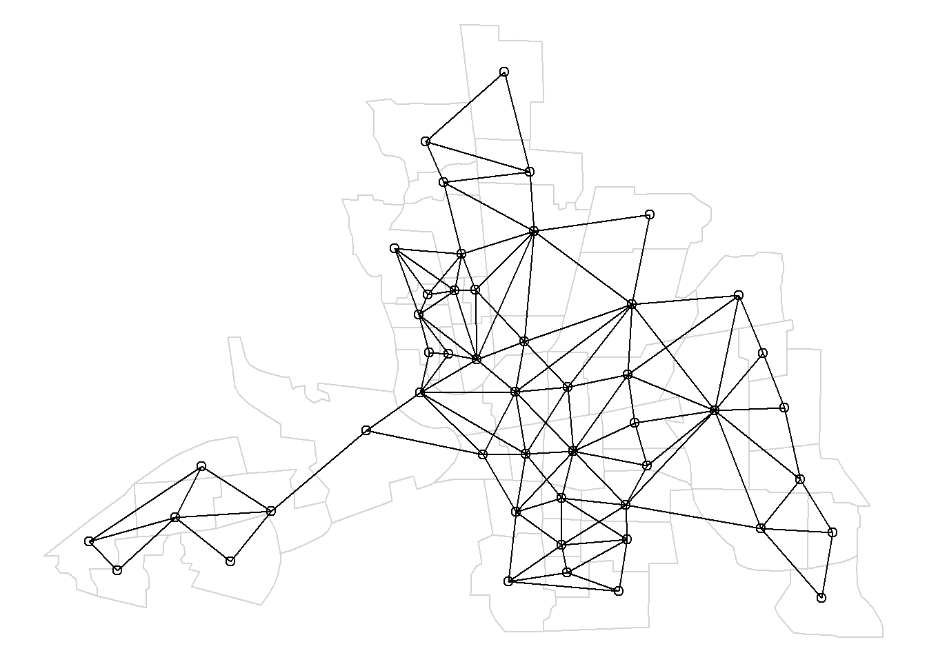

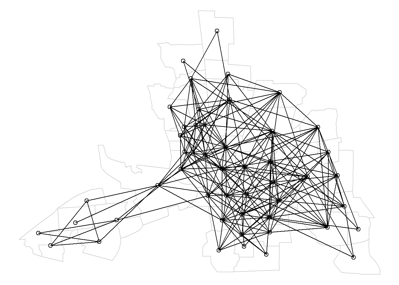
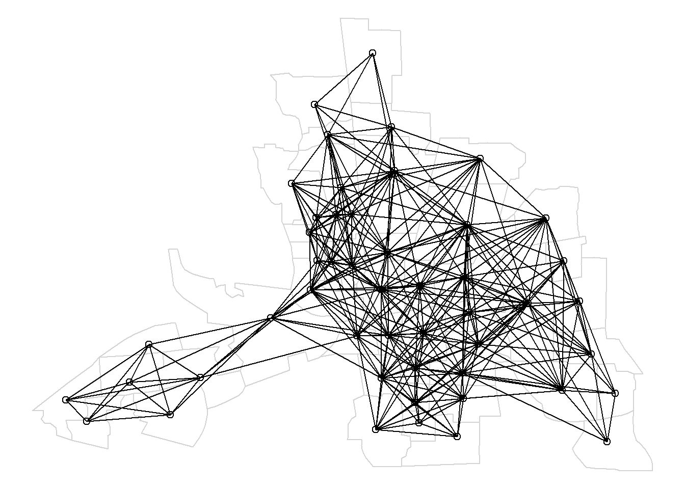
Figure 4.2: Map of neighbors based on contiguty. Neighbors of first order (left), second order (middle), and first order until second order (right).

5 Neighborhood matrices

A spatial neighborhood matrix \(W\) defines a neighborhood structure over the entire study region, and its elements can be viewed as weights. The \((i, j)\)th element of \(W\), denoted by \(w_{ij}\), spatially connects areas \(i\) and \(j\) in some fashion. More weight is associated with areas closer to \(i\) than those farther away from \(i\).

If neighbors are based on contiguity, we can construct a binary spatial matrix with \(w_{ij} = 1\) if regions \(i\) and \(j\) share a common boundary, and \(w_{ij} = 0\) otherwise. Customarily, \(w_{ii}\) is set to 0 for \(i = 1, \ldots, n\). An example of binary spatial matrix is shown in Figure 5.1. Note that this choice of proximity measure results in a symmetric spatial matrix.

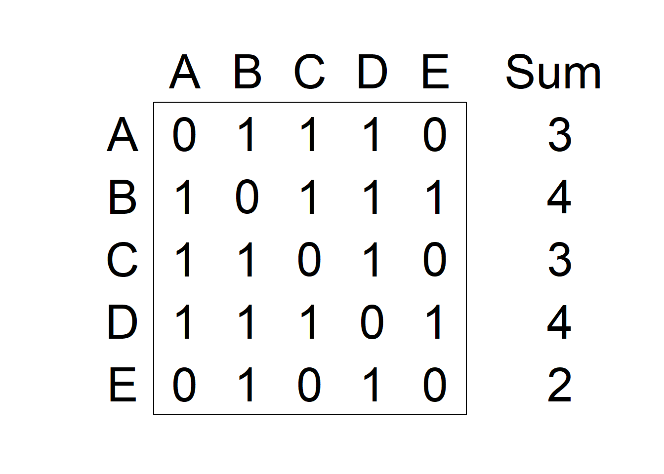
Figure 5.1: Left: Areas of the study region. Right: Spatial weight matrix calculated by assuming neighboring areas share a common boundary, and the sum of weights for each area.

Other spatial weight definitions could be to use \(w_{ij} = 1\) for all \(i\) and \(j\) within a specified distance, or to use \(w_{ij} = 1\) if \(j\) is one of the \(k\) nearest neighbors of \(i\). Weights \(w_{ij}\) can also be defined as the inverse distance between areas.

In addition, we may want to adjust for the total number of neighbors in each area and use a standardized matrix with entries \(w_{std,i,j} = w_{ij}/\sum_{j=1}^n w_{ij}\). Note that in most situations, this matrix is not symmetric when the areas are irregularly shaped.

5.1 Spatial weights matrix based on a binary neighbor list

The function nb2listw() of the spdep package can be used to construct a spatial neighborhood matrix containing the spatial weights corresponding to a neighbors list. The neighbors can be binary or based on inverse distance values. To compute a spatial weights matrix based on a binary neighbor list, we use the nb2listw() function with the following arguments:

• nb list with neighbors,
• style indicates the coding scheme chosen. For example, style = B is the basic binary coding, and W is row standardized (1/number of neighbors),
• zero.policy is used to take into account regions with 0 neighbors. Specifically, zero.policy = TRUE permits the weight list to contain zero-length weights vectors, and zero.policy = FALSE stops the function with an error if there are empty neighbor sets.

nb <- poly2nb(map, queen = TRUE)
nbw <- spdep::nb2listw(nb, style = "W")
head(nbw$weights)

## [[1]]
## [1] 0.5 0.5
## 
## [[2]]
## [1] 0.3333333 0.3333333 0.3333333
## 
## [[3]]
## [1] 0.25 0.25 0.25 0.25
## 
## [[4]]
## [1] 0.25 0.25 0.25 0.25
## 
## [[5]]
## [1] 0.125 0.125 0.125 0.125 0.125 0.125 0.125 0.125
## 
## [[6]]
## [1] 0.5 0.5

We can visualize the spatial weight matrix by creating a matrix with the weights with listw2mat(), and using lattice::levelplot() to create the plot (Figure 5.2).

m1 <- listw2mat(nbw)
lattice::levelplot(t(m1))

5.2 Spatial weights matrix based on inverse distance values

Given a list of neighbors, we can use nbdists() to compute the distances along the links. Then, we can construct the list with spatial weights based on inverse distance values using nb2listw() where the argument glist is equal to a list of general weights corresponding to neighbors. Figure 5.2 shows the spatial weight matrix obtained.

coo <- st_centroid(map)
nb <- poly2nb(map, queen = TRUE)
dists <- nbdists(nb, coo)
ids <- lapply(dists, function(x){1/x})
# head(ids)

nbw <- nb2listw(nb, glist = ids, style = "B")
head(nbw$weights)

## [[1]]
## [1] 1.670235 1.725073
## 
## [[2]]
## [1] 1.670235 1.404736 2.943309
## 
## [[3]]
## [1] 1.725073 1.404736 1.782670 1.910694
## 
## [[4]]
## [1] 2.943309 1.782670 1.448959 3.160865
## 
## [[5]]
## [1] 1.910694 1.448959 1.327423 1.914198 1.396239 2.159562 1.799038 1.322661
## 
## [[6]]
## [1] 1.327423 1.841662

m2 <- listw2mat(nbw)
lattice::levelplot(t(m2))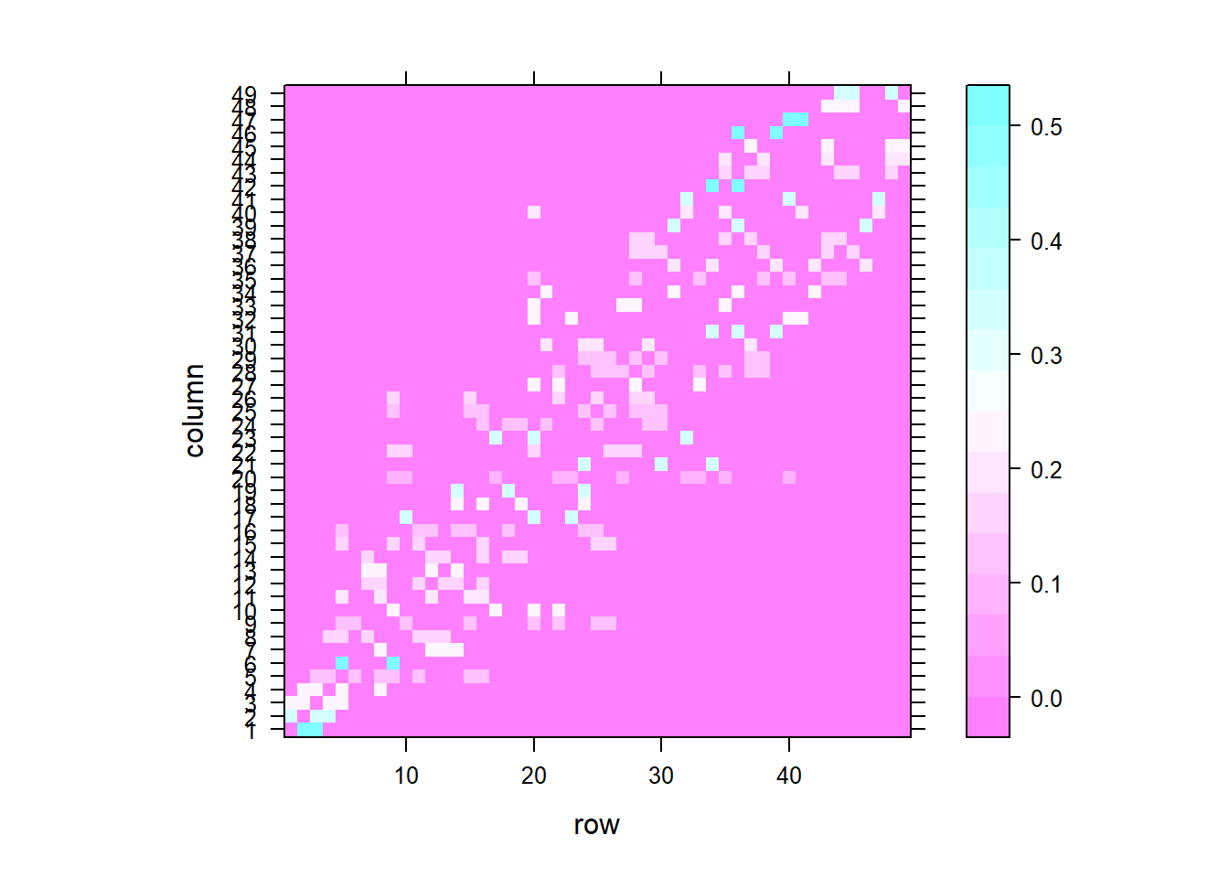

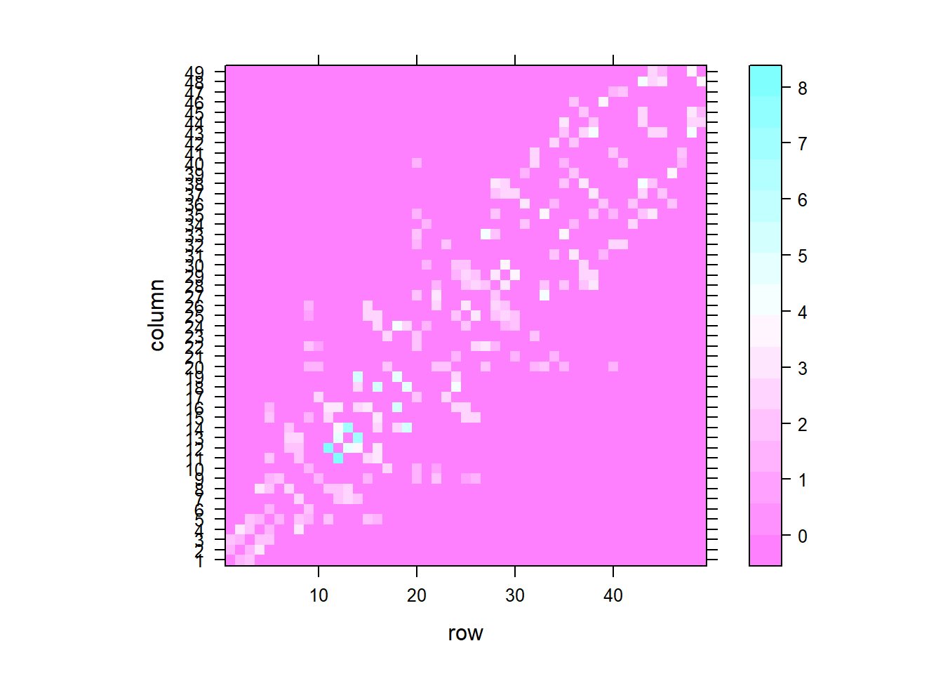
Figure 5.2: Spatial weights matrix based on binary neighbor list (left), and inverse distance values (right).

References

Bivand, Roger. 2022. Spdep: Spatial Dependence: Weighting Schemes, Statistics. https://CRAN.R-project.org/package=spdep.