R packages to download open spatial data
Paula Moraga, KAUST
Materials based on the book Geospatial Health Data (2019, Chapman & Hall/CRC)
http://www.paulamoraga.com/book-geospatial
Spatial data are used in a wide range of disciplines including environment, health, agriculture, economy and society. Several R packages have been recently developed as clients for various databases that can be used for easy access of spatial data including administrative boundaries, climatic, and OpenStreetMap data. Here, we give short reproducible examples on how to download and visualize spatial data that can be useful in different settings. More extended examples and details about the capabilities of each of the packages can be seen at the packages’ websites, and the rspatialdata website which provides a collection of tutorials on R packages to download and visualize spatial data using R.
1 Administrative boundaries of countries
We can download administrative boundaries of world countries with the packages rnaturalearth and rgeoboundaries. Other packages can also be used to obtain data of specific countries such as USA with tidycensus and tigris, Spain with mapSpain, and Brazil with geobr. The giscoR package helps to retrieve data from Eurostat - GISCO (the Geographic Information System of the COmmission) which contains several open data such as countries and coastal lines.
Here, we use rnaturalearth to download the administrative boundaries from Natural Earth map data.
Note that when installing rnaturalearth, we may get an error that can be fixed by installing the rnaturalearthhires package.
The ne_countries() function allows us to download the map of the country specified in argument country, of scale given in scale, and of class sp or sf given in returnclass.
We can retrieve the possible names that can be specified in argument country by typing ne_countries()$admin.
The ne_states() function can be used to obtain administrative divisions for specific countries.
Here, we download the maps of Germany and its divisions, and plot them side-by-side with the patchwork package.
# install.packages("devtools")
# devtools::install_github("ropensci/rnaturalearthhires")

library(rnaturalearth)
library(sf)
library(ggplot2)
library(viridis)
library(patchwork)

map1 <- ne_countries(type = "countries", country = "Germany", scale = "medium", returnclass = "sf")
map2 <- rnaturalearth::ne_states("Germany", returnclass = "sf")
p1 <- ggplot(map1) + geom_sf()
p2 <- ggplot(map2) + geom_sf()
p1 + p2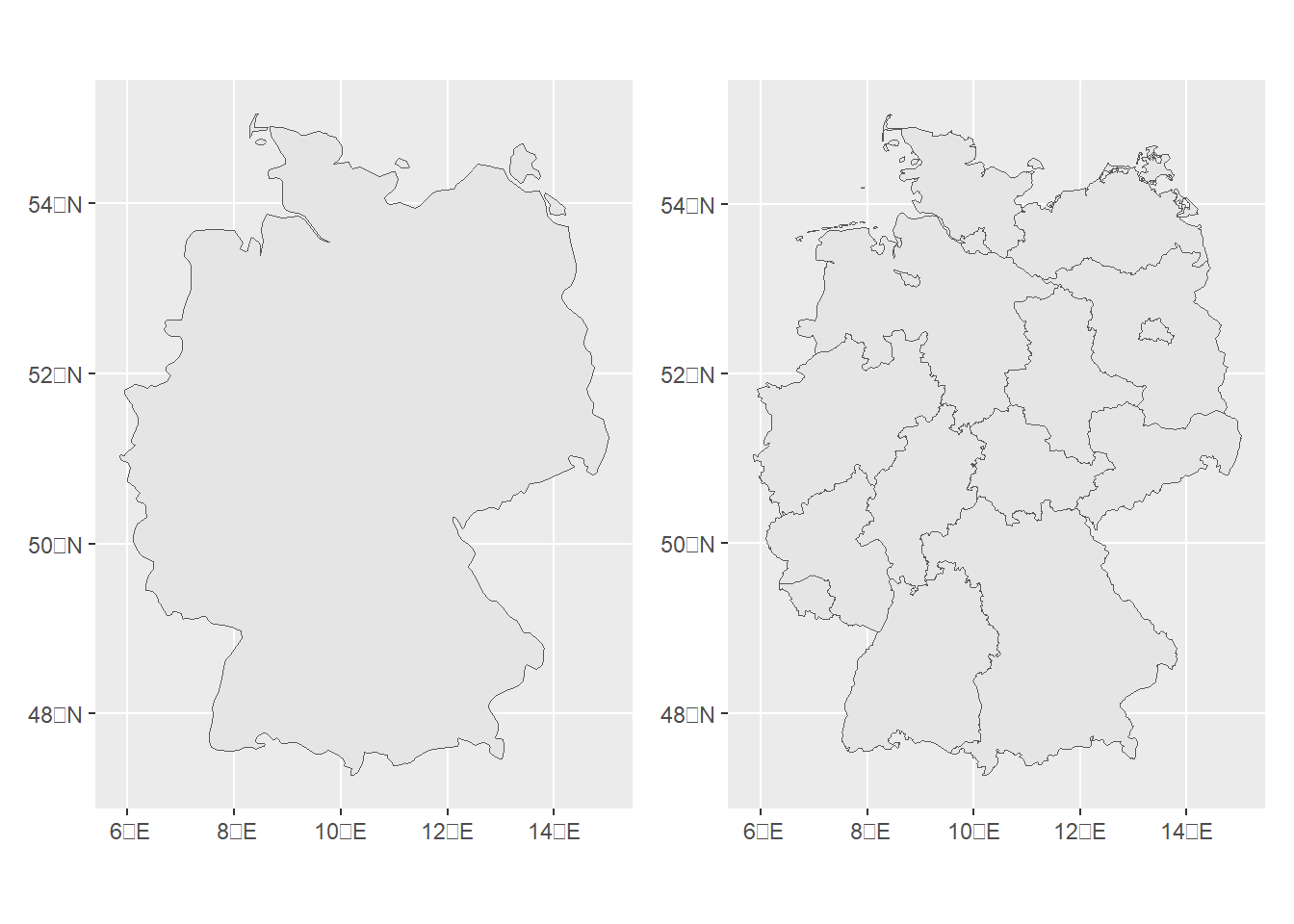
Note that if we needed maps of administrative boundaries at greater levels than the ones provided by these packages, we would need to resort to other sources such as online data repositories mantained by specific countries.
2 Climatic data
The geodata package allows us to download geographic data including climate, elevation, land use, soil, crop, species occurrence, administrative boundary and other data. The geodata package is a successor of the getData() function from the raster package.
For example, the worldclim_country() function downloads climate data from WorldClim including minimum temperature tmin, maximum temperature tmax, average temperature tavg, precipitation prec, and wind speed wind. The country_codes() function of geodata can be used to get the names and codes of the world countries. Here, we provide an example on how to download minimum temperature in Jamaica specifying country = "Jamaica" using tempdir() as the path name where to download the data. This function retrieves the temperature for each month and we can plot the mean over months with mean(d).
library(geodata)
d <- worldclim_country(country = "Jamaica", var = "tmin", path = tempdir())
terra::plot(mean(d), plg = list(title = "Min. temperature (C)"))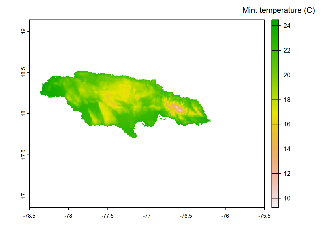
The geodata package can also be used to download other data such as elevation with elevation_30s(), land cover with landcover() or soil with soil_world().
3 Precipitation
The chirps package allows us to obtain daily high-resolution precipitation, as well as daily maximum and minimum temperatures from the Climate Hazards Group.
Here, we use the get_chirps() function to obtain daily precipitation in Bangkok, Thailand, by specifying the longitude and latitude coordinates of Bangkok, the dates and the server.
The default server is "CHC". Here, we use the "ClimateSERV" server which is recommended when few data-points are required.
library("chirps")
location <- data.frame(long = 100.523186, lat = 13.736717)
d <- get_chirps(location, dates = c("2020-01-01", "2022-12-31"), server = "ClimateSERV")
ggplot(d, aes(x = date, y = chirps)) + geom_line() + labs(y = "Precipitation (mm)")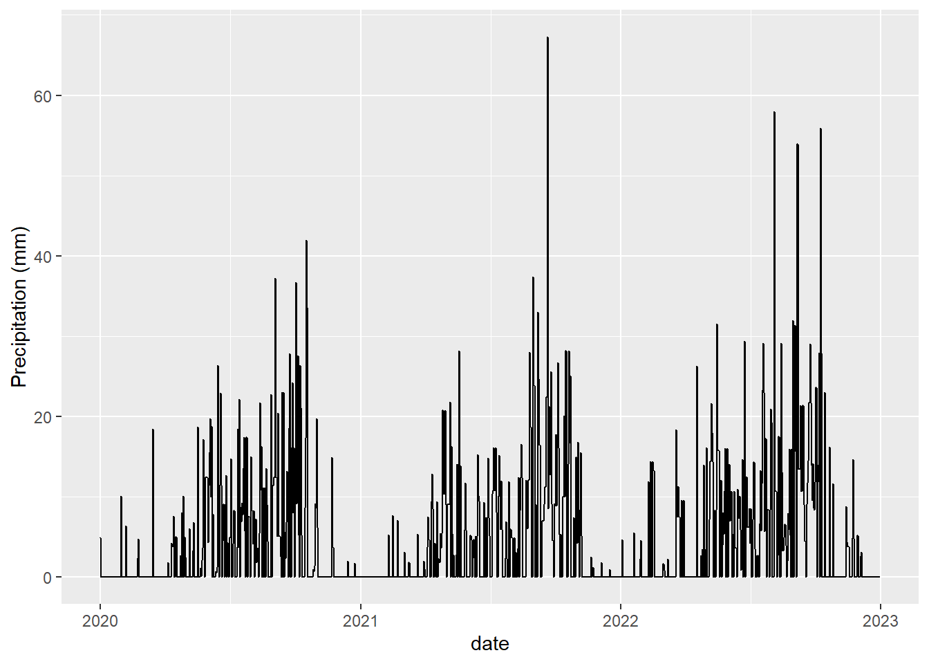
4 Elevation
The elevatr package allows us to get elevation data from Amazon Web Services (AWS) Terrain Tiles and OpenTopography Global Digital Elevation Models API.
The get_elev_raster() function can be used to download elevation at the locations specified in argument locations and with a zoom specified in argument z.
Argument clip can be set to "tile" to return full tiles, "bbox" to return data clipped to the bounding box of the locations, or "locations" to return data clipped to the data specified in locations.
Here, we download the altitude of Switzerland passing an sf object with the map of the country.
library(rnaturalearth)
library(elevatr)
library(terra)
map <- ne_countries(type = "countries", country = "Switzerland", scale = "medium", returnclass = "sf")
d <- get_elev_raster(locations = map, z = 9, clip = "locations")
terra::plot(rast(d), plg = list(title = "Elevation (m)"))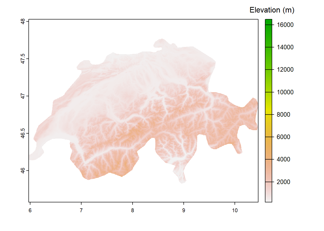
5 OpenStreetMap data
OpenStreetMap (OSM) is an open world geographic database updated and maintained by a community of volunteers.
We can use the osmdata package to retrieve OSM data including roads, shops, railway stations and much more. The available_features() function can be used to get the list of recognized features in OSM. This list can be found in the OSM wiki.
library(osmdata)
head(available_features())
## [1] "4wd_only" "abandoned" "abutters" "access" "addr" "addr:city"The available_tags() function lists out the tags associated with each feature. For example, tags associated with feature "amenity" can be obtained as follows:
head(available_tags("amenity"))## [1] "animal_boarding" "animal_breeding" "animal_shelter" "animal_training"
## [5] "arts_centre" "atm"The first step in creating an osmdata query is defining the geographical area we wish to include in the query. This can be done by defining a bounding box that defines a geographical area by its bounding latitudes and longitudes. The bounding box for a given place name can be obtained with the getbb() function. For example, the bounding box of Barcelona, Spain, can be obtained as follows.
placebb <- getbb("Barcelona")
placebb
## min max
## x 2.052498 2.228356
## y 41.317035 41.467914To retrieve the required features of a place defined by the bounding box, we need to create an overpass query with opq().
Then, the add_osm_feature() function can be used to add the required features to the query. Finally, we use the osmdata_sf() function to obtain a simple feature object of the resultant query. For example, we can obtain the hospitals of Barcelona specifying its bounding box placebb and using add_osm_feature() with key = "amenity" and value = "hospital" as follows.
hospitals <- placebb %>% opq() %>%
  add_osm_feature(key = "amenity", value = "hospital") %>% osmdata_sf()
Motorways can be retrieved using key = "highway and value = "motorway".
motorways <- placebb %>% opq() %>%
  add_osm_feature(key = "highway", value = "motorway") %>% osmdata_sf()
We can visualize an interactive map of the hospitals and motorways of Barcelona as follows.
library(leaflet)
leaflet() %>%  addTiles() %>%
  addPolylines(data = motorways$osm_lines, color = "black") %>%
  addPolygons(data = hospitals$osm_polygons, label = hospitals$osm_polygons$name)
6 World Bank data
The World Bank provides a great source of global socio-economic data spanning several decades and dozens of topics, with the potential to shed light on numerous global issues. Some of the indicators can be seen at this website.
The wbstats package allows us to search and download data from the World Bank API.
The wb_search() function can be used to find indicator that match a search term. For example, we can find indicators that contain the world "poverty", "unemployment" or "employment" as follows.
library(wbstats)
indicators <- wb_search(pattern = "poverty|unemployment|employment")
# print(indicators)
We can inspect the indicators retrieved with View(indicators).
The function wb_data() allows us to retrieve the chosen data. For example, here we download Human Development Index which has ID MO.INDEX.HDEV.XQ in 2011.
d <- wb_data(indicator = "MO.INDEX.HDEV.XQ", start_date = 2011, end_date = 2011)
print(head(d))
## # A tibble: 6 × 9
## iso2c iso3c country date MO.IN…¹ unit obs_s…² footn…³ last_upd…⁴
## <chr> <chr> <chr> <dbl> <dbl> <chr> <chr> <chr> <date>
## 1 AO AGO Angola 2011 47.7 <NA> <NA> <NA> 2013-02-22
## 2 BI BDI Burundi 2011 48.5 <NA> <NA> <NA> 2013-02-22
## 3 BJ BEN Benin 2011 53.2 <NA> <NA> <NA> 2013-02-22
## 4 BF BFA Burkina Faso 2011 45.8 <NA> <NA> <NA> 2013-02-22
## 5 BW BWA Botswana 2011 80.3 <NA> <NA> <NA> 2013-02-22
## 6 CF CAF Central African Re… 2011 32.9 <NA> <NA> <NA> 2013-02-22
## # … with abbreviated variable names ¹MO.INDEX.HDEV.XQ, ²obs_status, ³footnote,
## # ⁴last_updatedWe can visualize a map with the data by adding the data d to a map of Africa retrieved with the ne_countries() function of rnaturalearth.
library(rnaturalearth)
library(mapview)
map <- ne_countries(continent = "Africa", returnclass = "sf")
map <- dplyr::left_join(map, d, by = c("iso_a3" = "iso3c"))
mapview(map, zcol = "MO.INDEX.HDEV.XQ")
7 Species occurrence
The spocc package is an interface to many species occurrence data sources including Global Biodiversity Information Facility (GBIF), USGSs’ Biodiversity Information Serving Our Nation (BISON), iNaturalist, eBird, Integrated Digitized Biocollections (iDigBio), VertNet, Ocean Biogeographic Information System (OBIS), and Atlas of Living Australia (ALA). The package provides functionality to retrieve and combine species occurrence data.
The occ() function from spocc can be used to retrieve the locations of species.
Here, we download data on brown-throated sloths in Costa Rica recorded between 2000 and 2019 from the GBIF database.
Arguments of this function include query with the species scientific name (Bradypus variegatus), from with the name of the database (GBIF), and date with the start and end dates (2000-01-01 to 2019-12-31). We also specify we wish to retrieve occurrences in Costa Rica by setting gbifopts to a named list with country equal to the 2-letter code of Costa Rica (CR). Moreover, we only retrieve occurrence data that have coordinates by setting has_coords = TRUE, and specify limit equal to 1000 to retrieve a maximum of 1000 occurrences.
library('spocc')
df <- occ(query = 'Bradypus variegatus', from = 'gbif', date = c("2000-01-01", "2019-12-31"),
          gbifopts = list(country = "CR"), has_coords = TRUE, limit = 1000)
d <- occ2df(df)
Then, we transform the point data to an sf object with st_as_sf(), assign the coordinate reference system given by the EPSG code 4326 to represent longitude and latitude coordinates, and visualize it with mapview.
library(sf)
d <- st_as_sf(d, coords = c("longitude", "latitude"))
st_crs(d) <- 4326
mapview(d)
8 Population, health and other spatial data
Other packages that can be used to obtain spatial data for the world or specific countries include the following. The wopr package provides access to the WorldPop Open Population Repository and provides estimates of population sizes for specific geographic areas. These data is collected by the WorldPop Hub (https://hub.worldpop.org/) which provides open high-resolution geospatial data on population count and density, demographic and dynamics, with a focus on low- and middle- income countries.
The rdhs package gives the users the ability to access and make analysis on the Demographic and Health Survey (DHS) data. The malariaAtlas package can be used to download, visualize and manipulate global malaria data hosted by the Malaria Atlas Project.
The openair package allows us to obtain air quality data and other atmospheric composition data.
The rtweet package can be used to collect Twitter data. This package provides an implementation of calls designed to collect and organize Twitter data via Twitter’s REST and stream Application Program Interfaces (API), which can be found at the following URL.
Many other spatial datasets are included in several packages mainly to demonstrate the packages’ functionality.
For example, spatstat contains point pattern data that can be listed with data(package="spatstat.data").
The spData package also includes diverse spatial datasets that can be used for teaching spatial data analysis.
R also has packages that allow us to geocode place names or addresses. For example, the packages ggmap and opencage can be used to convert names to geographic coordinates.