The sf package for spatial vector data
Paula Moraga, KAUST
Materials based on the book Geospatial Health Data (2019, Chapman & Hall/CRC)
http://www.paulamoraga.com/book-geospatial
1 Simple features (sf)
The sf package (Pebesma 2022) can be used to represent and work with vector spatial data including points, polygons and lines, and their associated information.
The sf package uses sf objects that are extensions of data frames containing a collection of simple features or spatial objects with possibly associated data.
We can read an sf object with the st_read() function of sf.
For example, here we read the nc shapefile of sf which contains the counties of North Carolina, USA, as well as their name, number of births, and number of sudden infant deaths in 1974 and 1979.
library(sf)
pathshp <- system.file("shape/nc.shp", package = "sf")
nc <- st_read(pathshp, quiet = TRUE)
class(nc)
## [1] "sf" "data.frame"The sf object nc is a data.frame containing a collection with 100 simple features (rows) and 6 attributes (columns) plus a list-column with the geometry of each feature. An sf object contains the following objects of class sf, sfc and sfg:
sf(simple feature): each row of thedata.frameis a single simple feature consisting of attributes and geometry.sfc(simple feature geometry list-column): thegeometrycolumn of thedata.frameis a list-column of classsfcwith the geometry of each simple feature.sfg(simple feature geometry): each of the rows of thesfclist-column corresponds to the simple feature geometry (sfg) of a single simple feature.
We can see and plot the information of the sf object as follows (Figure 1.1):
print(nc)## Simple feature collection with 100 features and 14 fields
## Geometry type: MULTIPOLYGON
## Dimension: XY
## Bounding box: xmin: -84.32385 ymin: 33.88199 xmax: -75.45698 ymax: 36.58965
## Geodetic CRS: NAD27
## First 10 features:
## AREA PERIMETER CNTY_ CNTY_ID NAME FIPS FIPSNO CRESS_ID BIR74 SID74
## 1 0.114 1.442 1825 1825 Ashe 37009 37009 5 1091 1
## 2 0.061 1.231 1827 1827 Alleghany 37005 37005 3 487 0
## 3 0.143 1.630 1828 1828 Surry 37171 37171 86 3188 5
## 4 0.070 2.968 1831 1831 Currituck 37053 37053 27 508 1
## 5 0.153 2.206 1832 1832 Northampton 37131 37131 66 1421 9
## 6 0.097 1.670 1833 1833 Hertford 37091 37091 46 1452 7
## 7 0.062 1.547 1834 1834 Camden 37029 37029 15 286 0
## 8 0.091 1.284 1835 1835 Gates 37073 37073 37 420 0
## 9 0.118 1.421 1836 1836 Warren 37185 37185 93 968 4
## 10 0.124 1.428 1837 1837 Stokes 37169 37169 85 1612 1
## NWBIR74 BIR79 SID79 NWBIR79 geometry
## 1 10 1364 0 19 MULTIPOLYGON (((-81.47276 3...
## 2 10 542 3 12 MULTIPOLYGON (((-81.23989 3...
## 3 208 3616 6 260 MULTIPOLYGON (((-80.45634 3...
## 4 123 830 2 145 MULTIPOLYGON (((-76.00897 3...
## 5 1066 1606 3 1197 MULTIPOLYGON (((-77.21767 3...
## 6 954 1838 5 1237 MULTIPOLYGON (((-76.74506 3...
## 7 115 350 2 139 MULTIPOLYGON (((-76.00897 3...
## 8 254 594 2 371 MULTIPOLYGON (((-76.56251 3...
## 9 748 1190 2 844 MULTIPOLYGON (((-78.30876 3...
## 10 160 2038 5 176 MULTIPOLYGON (((-80.02567 3...plot(nc)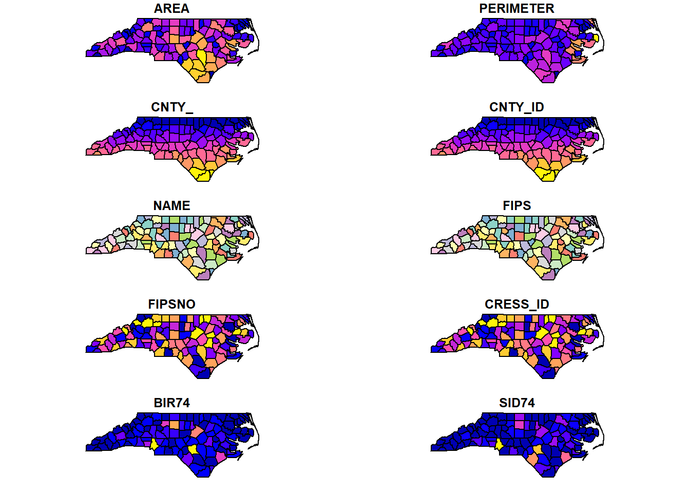
Figure 1.1: sf object representing the counties of North Carolina, USA, and associated information.
We can subset feature sets by using the square bracket notation,
and use the drop argument to drop geometries.
nc[1, ] # first row
nc[nc$NAME == "Ashe", ] # row with NAME "Ashe"
nc[1, "NWBIR74"] # first row, column with name NWBIR74
nc[1, "NWBIR74", drop = TRUE] # drop geometry
The st_geometry() function can be used to retrieve
the simple feature geometry list-column (sfc).
# Geometries printed in abbreviated form
st_geometry(nc)
# View complete geometry by selecting one
st_geometry(nc)[[1]]
2 Creating an sf object
We can use the st_sf() function to create an sf object by providing two elements, namely,
a data.frame with the attributes of each feature, and
a simple feature geometry list-column sfc containing simple feature geometries sfg.
In more detail, we create simple feature geometries sfg and use the st_sfc() function to create a simple feature geometry list-column sfc with them. Then, we use st_sf() to put the data.frame with the attributes and the simple feature geometry list-column sfc together.
Simple feature geometries sfg objects can be, for example, of type POINT (single point), MULTIPOINT (set of points) or POLYGON (polygon), and can be created with st_point(), st_multipoint() and st_polygon(), respectively.
Figure 2.1 shows an example of sf objects representing a single point, a set of points and a polygon created with the following code:
# Single point (point as a vector)
x <- st_point(c(1, 2))

# Set of points (points as a matrix)
p <- rbind(c(3.2, 4), c(3, 4.6), c(3.8, 4.4),
           c(3.5, 3.8), c(3.4, 3.6), c(3.9, 4.5))
mp <- st_multipoint(p)

# Polygon. Sequence of points that form a closed,
# non-self intersecting ring.
# The first ring denotes the exterior ring,
# zero or more subsequent rings denote holes in the exterior ring
p1 <- rbind(c(0, 0), c(1, 0), c(3, 2), c(2, 4), c(1, 4), c(0, 0))
p2 <- rbind(c(1, 1), c(1, 2), c(2, 2), c(1, 1))
pol <- st_polygon(list(p1, p2))

# Plot single point, set of points and polygon
plot(x, main = "POINT")
plot(mp, main = "MULTIPOINT")
plot(pol, main = "POLYGON")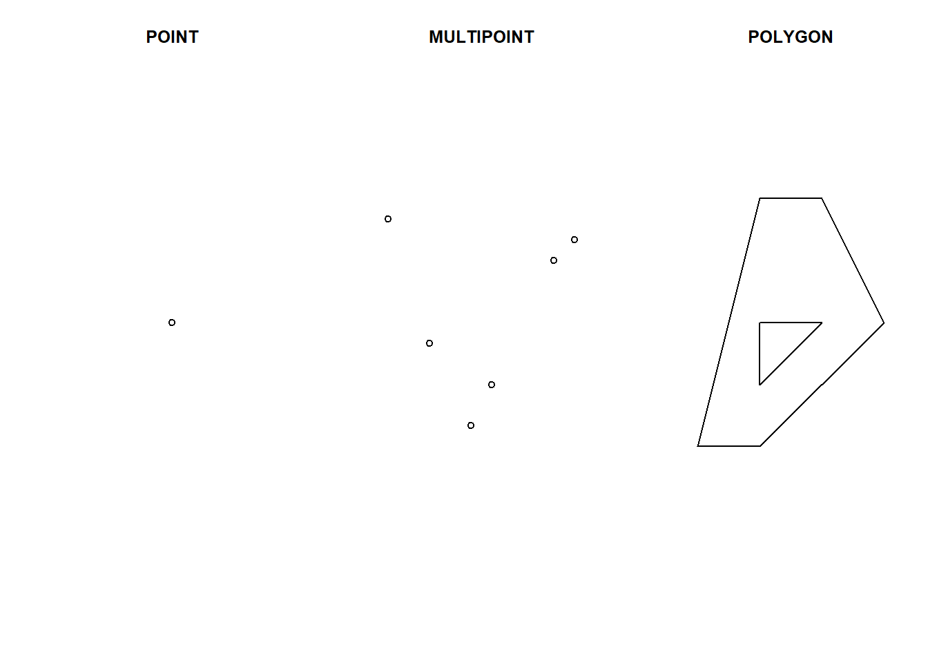
Figure 2.1: sf objects representing a single point, a set of points and a polygon.
Here, we create an sf object containing three points with two attributes.
First, we create three simple feature geometry objects (sfg) of type POINT using st_point().
Then, we use st_sfc() to create a simple feature geometry list-column sfc with the sfg objects.
Finally, we use st_sf() to put the data.frame with the attributes and the simple feature geometry list-column sfc together.
Figure 2.2 shows the resulting object plotted with ggplot2 (Wickham, Chang, et al. 2022).
p1_sfg <- st_point(c(1, 1))
p2_sfg <- st_point(c(2, 2))
p3_sfg <- st_point(c(3, 3))
p_sfc <- st_sfc(p1_sfg, p2_sfg, p3_sfg)
df <- data.frame(v1 = c("A", "B", "C"), v2 = as.factor(c(10, 20, 20)))
p_sf <- st_sf(df, geometry = p_sfc)

library(ggplot2)
ggplot(p_sf) + geom_sf(aes(shape = v1, col = v2), size = 6) + theme_bw()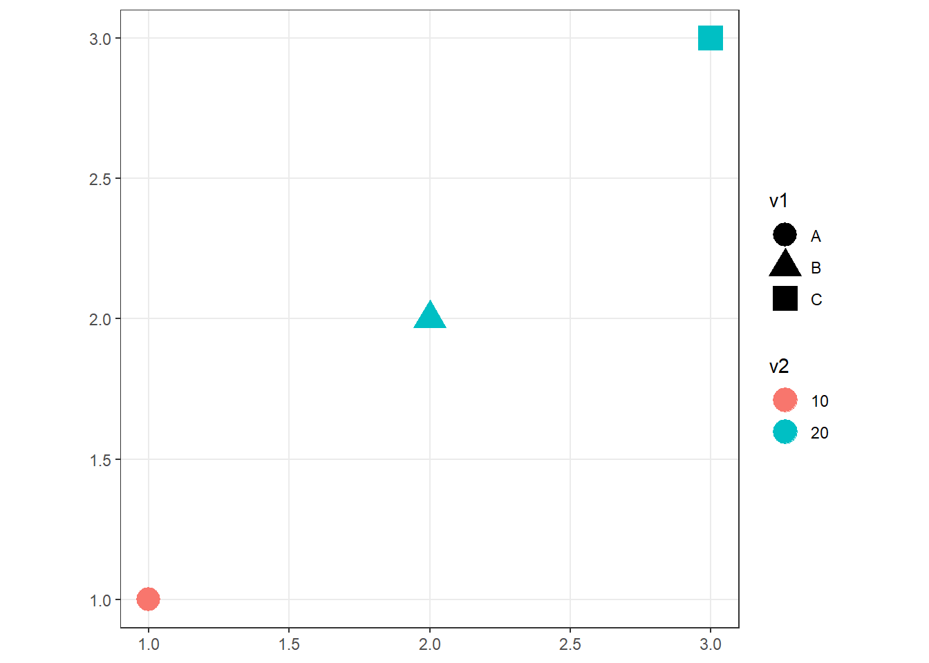
Figure 2.2: sf object representing a set of points and associated attributes.
3 st_*() functions
Common functions to manipulate sf objects include the following:
st_read()reads ansfobject,st_write()writes ansfobject,st_crs()gets or sets new coordinate reference systems (CRS),st_transform()transforms data to a new CRS,st_intersection()intersectssfobjects,st_union()combines severalsfobjects into one,st_simplify()simplifies ansfobject,st_coordinates()retrieves coordinates of ansfobject,st_as_sf()converts a foreign object to ansfobject.
For example, we can read an sf object as follows:
library(sf)
library(ggplot2)
map <- read_sf(system.file("shape/nc.shp", package = "sf"))
We can inspect the first rows of the sf object map with head().
head(map)We can delete some of the polygons by taking a subset of the rows of map (Figure 3.1).
map <- map[-which(map$FIPS %in% c("37125", "37051")), ]
ggplot(map) + geom_sf(aes(fill = SID79))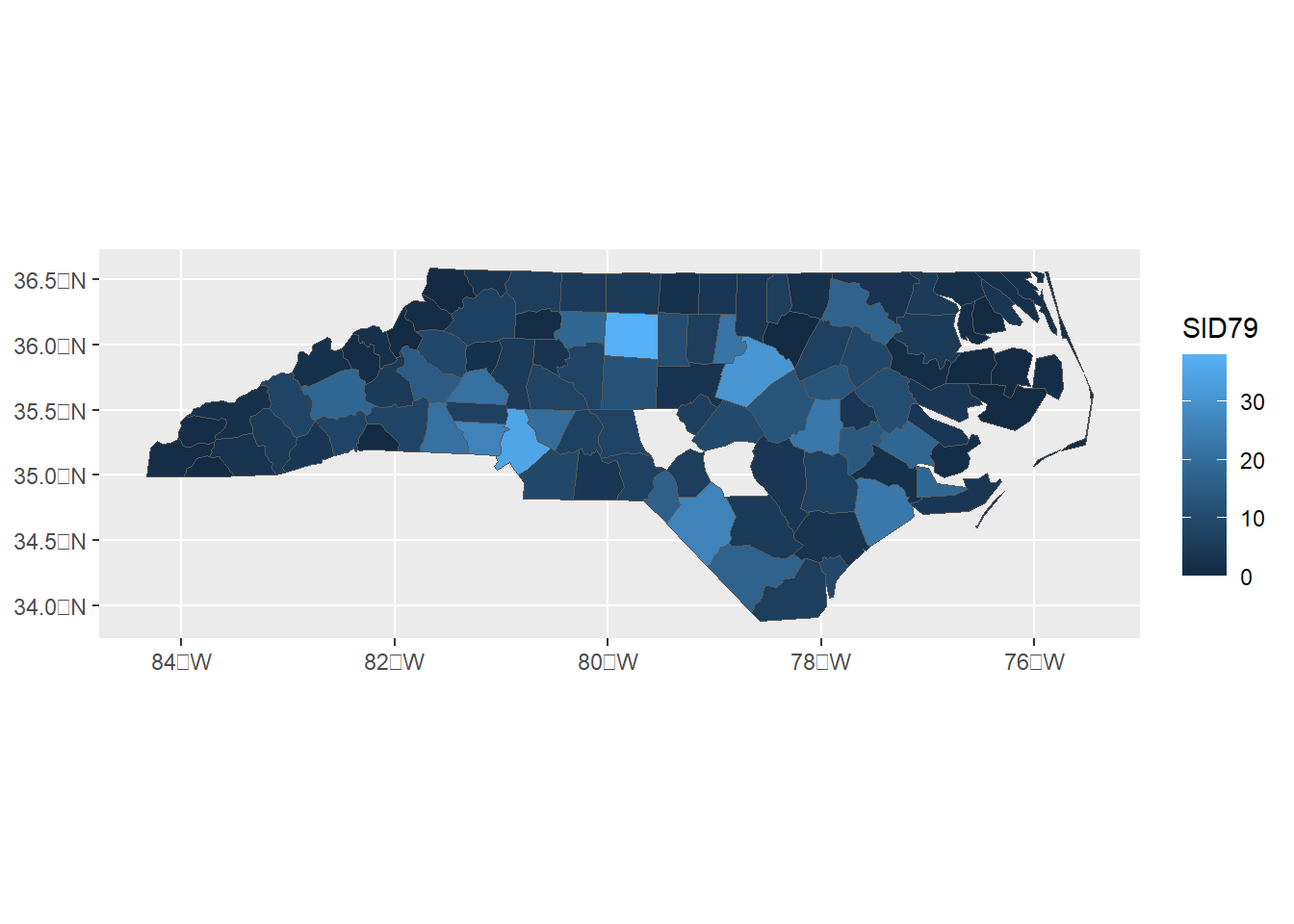
Figure 3.1: sf object obtained by deleting some polygons.
We can use st_union() with argument by_feature = FALSE to combine all geometries together (Figure 3.2).
ggplot(st_union(map, by_feature = FALSE) %>% st_sf()) + geom_sf()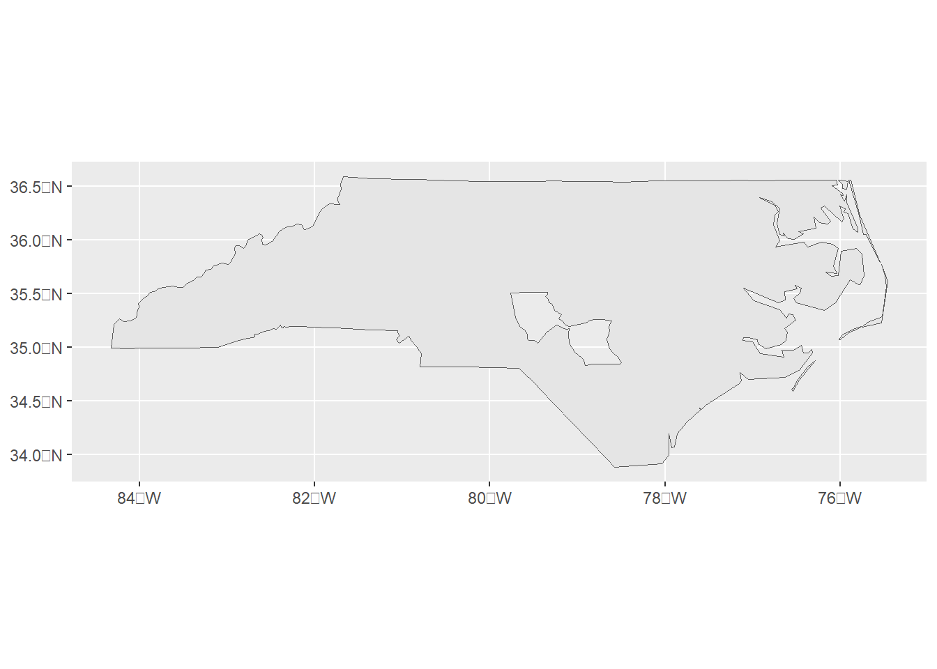
Figure 3.2: sf object obtained by combining polygons.
Figure 3.3 shows the map obtained by simplifying the boundaries with the st_simplify() function.
ggplot(st_simplify(map, dTolerance = 10000)) + geom_sf()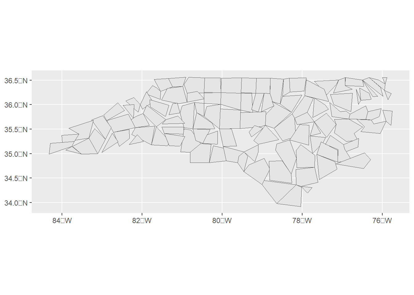
Figure 3.3: sf object obtained by simplifying polygons.
4 Transforming point data to an sf object
The st_as_sf() function allows us to convert a foreign object to an sf object.
For example, we can have a data frame containing the coordinates of a number of locations and attributes that we wish to turn into an sf object.
To do that, we use the st_as_sf() function passing the object we wish to convert and specifying in argument coords the name of the columns that contain the point coordinates. For example, here we use st_as_sf() to turn a data frame containing coordinates long and lat and two variables place and value to an sf object.
Then, we use st_crs() to set the coordinate reference system given by the EPSG code 4326 to represent longitude and latitude coordinates.
Figure 4.1 shows the plot of the sf object obtained with mapview (Appelhans et al. 2022).
library(sf)
library(mapview)

d <- data.frame(
place = c("London", "Paris", "Madrid", "Rome"),
long = c(-0.118092, 2.349014, -3.703339, 12.496366),
lat = c(51.509865, 48.864716, 40.416729, 41.902782),
value = c(200, 300, 400, 500))
class(d)
## [1] "data.frame"dsf <- st_as_sf(d, coords = c("long", "lat"))
st_crs(dsf) <- 4326
class(dsf)## [1] "sf" "data.frame"mapview(dsf)
Figure 4.1: sf object with points.
5 Counting the number of points within polygons
We can use the st_intersects() function of sf to count the number of points within the polygons of an sf object (Figure 5.1).
The returned object is a list with feature ids intersected in each of the polygons.
We can use the lengths() function to calculate the number of points inside each feature as seen in Figure 5.2.
library(sf)
library(ggplot2)

# Map with divisions (sf object)
map <- read_sf(system.file("shape/nc.shp", package = "sf"))

# Points over map (simple feature geometry list-column sfc)
points <- st_sample(map, size = 1000)

# Map. reset = FALSE to add further map elements
plot(map[, 1], reset = FALSE, col = "grey")
plot(points, add = TRUE)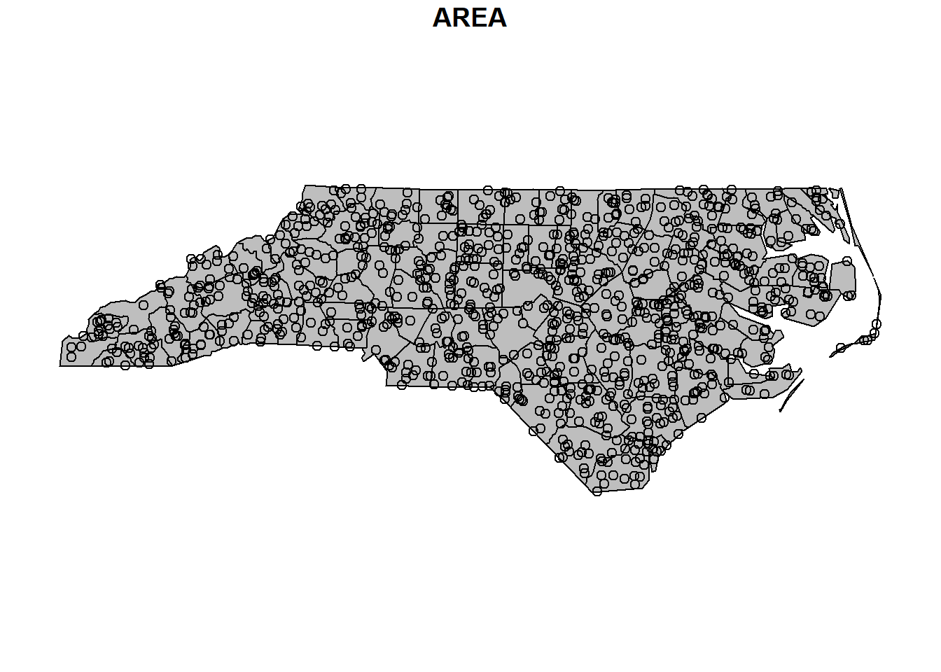
Figure 5.1: Points within polygons.
# Intersection (first argument map, then points)
inter <- st_intersects(map, points)

# Add point count to each polygon
map$count <- lengths(inter)

# Map
ggplot(map) + geom_sf(aes(fill = count))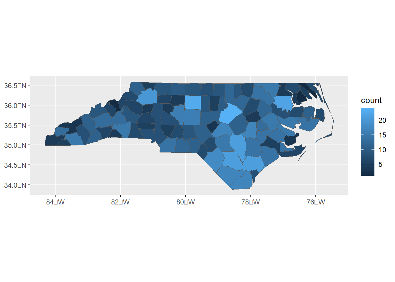
Figure 5.2: Number of points within polygons.
6 Identifying polygons containing points
Given an sf object with points and an sf object with polygons,
we can also use the st_intersects() function to obtain the polygon each of the points belong to. For example, Figure 6.1 shows a map with the names of the polygons that contain three points over the map.
library(sf)
library(ggplot2)

# Map with divisions (sf object)
map <- read_sf(system.file("shape/nc.shp", package = "sf"))

# Points over map (sf object)
points <- st_sample(map, size = 3) %>% st_as_sf()

# Intersection (first argument points, then map)
inter <- st_intersects(points, map)

# Adding column arename with the name of
# the areas containing the points
points$areaname <- map[unlist(inter), "NAME",
                       drop = TRUE] # drop geometry
points
# Map
ggplot(map) + geom_sf() + geom_sf(data = points) +
geom_sf_label(data = map[unlist(inter), ],
aes(label = NAME), nudge_y = 0.2)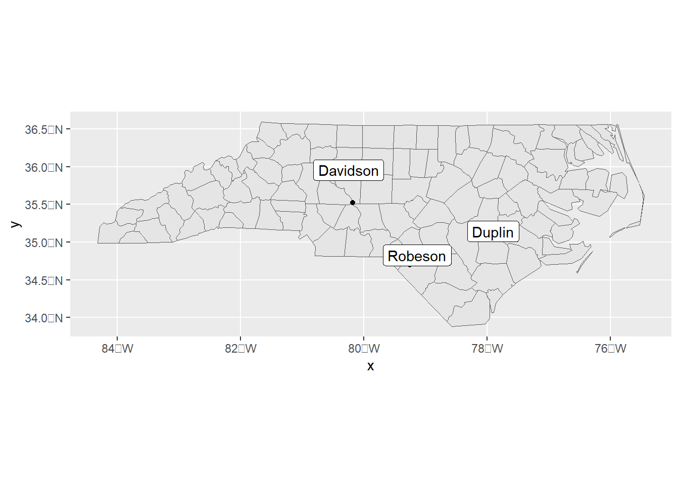
Figure 6.1: Map showing the name of polygons that contain three points over the map.
7 Joining map and data
Sometimes, a map and its corresponding data are available separately and we may wish to create an sf object representing the map with the added data that we can manipulate and plot.
We can create an sf map with the data attributes by joining the map and the data with the left_join() function of the dplyr (Wickham, François, et al. 2022) package.
Here, we present an example where we add air pollution data obtained with the wbstats (Piburn 2020) package to an sf map obtained with the rnaturalearth package.
First, we use the ne_countries() function of rnaturalearth (South 2017) to download the world country polygons of class sf.
# Map
library(rnaturalearth)
map <- ne_countries(returnclass = "sf")
Then, we use the wbstats package to download a data frame of air pollution data from the World Bank. Specifically, we search the pollution indicators with wb_search(), and use wb_data() to download PM2.5 in year 2016 by specifying the indicator corresponding to PM2.5, and the start and end dates.
# Data
library(wbstats)
indicators <- wb_search(pattern = "pollution")
d <- wb_data(indicator = "EN.ATM.PM25.MC.M3",
             start_date = 2016, end_date = 2016)
head(d)
Then, we use the left_join() function of dplyr to join the map and the data specifying in the argument by the variables we wish to join by. Here, we use ISO3 standard code of the countries rather than the country names since names can be written differently in the map and the data frame. Figure 7.1 shows the map of the data obtaind with ggplot2.
# Join
library(dplyr)
map1 <- left_join(map, d, by = c("iso_a3" = "iso3c"))

# Plot
library(ggplot2)
library(viridis)
ggplot(map1) + geom_sf(aes(fill = EN.ATM.PM25.MC.M3)) +
  scale_fill_viridis() + theme_bw()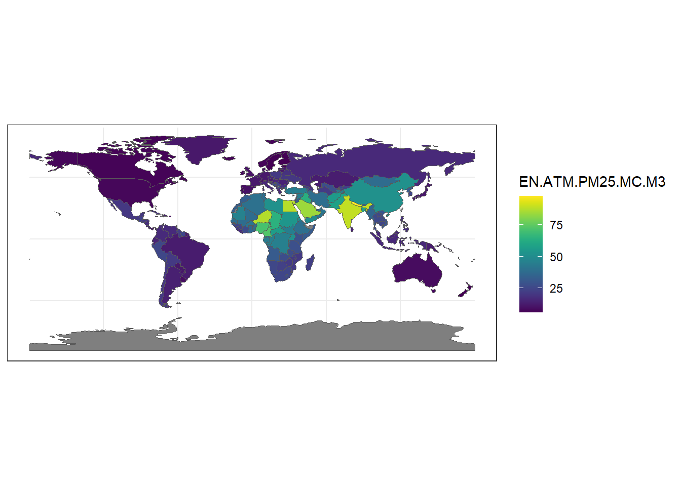
Figure 7.1: PM2.5 values in each of the world countries in 2016.
Note that when we use left_join(), the class of the resulting object is be the same as the class of the first argument. Thus, left_join(sf_object, data.frame_object) creates an sf object, whereas
left_join(data.frame_object, sf_object) is a data.frame:
map1 <- left_join(map, d, by = c("iso_a3" = "iso3c"))
class(map1)
## [1] "sf" "data.frame"d1 <- left_join(d, map, by = c("iso3c" = "iso_a3"))
class(d1)## [1] "tbl_df" "tbl" "data.frame"Note that given two data frames x and y, we can join them by using the left_join(), right_join(), inner_join() or full_join() functions.
Specifically, left_join(x, y) includes all rows in x so the resulting data frame includes all observations in the left data frame x, whether or not there is a match in the right data frame y.
right_join(x, y) includes all rows in y so the resulting data frame includes all observations in y, whether or not there is a match in x.
inner_join(x, y) includes all rows in x and y so the resulting data frame includes only observations that are in both data frames.
Finally, full_join(x, y) includes all rows in x or y so the resulting data frame includes all observations from both data frames.