Spatial data in R
Paula Moraga, KAUST
Materials based on the book Geospatial Health Data (2019, Chapman & Hall/CRC)
http://www.paulamoraga.com/book-geospatial
Spatial data can be represented using vector and raster data. Vector data is used to display points, lines and polygons, and possibly their associated information. Vector data may represent, for example, locations of monitoring stations, road networks, or municipalities of a country. Raster data are regular grids with cells of equal size that are used to store values of spatially continuous phenomena, such as elevation, temperature or air pollution values.
The sf (Pebesma 2022a) and terra (Hijmans 2022) packages are the main packages that allow us to manipulate and analyze spatial data in R. In this tutorial, we introduce these packages, spatial data storage files, and coordinate reference systems. Finally, we give an overview of old spatial packages that were widely used but are not longer maintained.
1 Vector data
The sf package allows us to work with vector data which is used to represent points, lines and polygons (Figure 1.1). Vector data can be used, for example, to represent locations of hospitals or monitoring stations as points, roads or rivers as lines, and municipalities or districts of a country as polygons. Moreover, these data can also have associated information such as temperature values measured at monitoring stations or number of people living in municipalities.
Before the sf package was developed, the sp package (Pebesma and Bivand 2022), which is not longer maintained, was used to work with vector spatial data. The terra package presented in the following sections is mainly used to work with rasters and also has functionality to work with vector data.
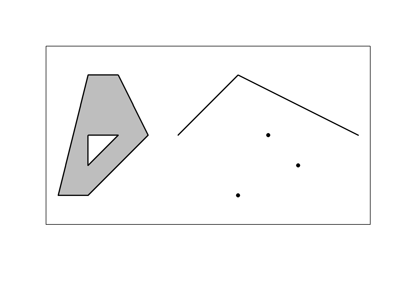
Figure 1.1: Examples of vector data (points, line and polygon).
1.1 Shapefile
Vector data are often represented using a data storage format called shapefile. Note that a shapefile is not a single file but a collection of related files.
A shapefile has three mandatory files, namely,
.shp which contains the geometry data,
.shx which is a positional index of the geometry data that allows to seek forwards and backwards the .shp file,
and .dbf which stores the attributes for each shape.
Other files that may form a shapefile include
.prj which is a plain text file describing the projection,
.sbn and .sbx which are spatial indices of the geometry data,
and .shp.xml which contains spatial metadata in XML format.
Therefore, when working with a shapefile, it is important to obtain all files that compose the shapefile and not only the .shp file with the geometry data.
The st_read() function of the sf package can be used to read a shapefile.
Here, we read the shapefile of the counties of North Carolina, USA, contained in the sf package.
First, we use system.file() passing the name of the directory ("shape/nc.shp") and the name of the package ("sf") to identify the path of shapefile.
library(sf)
pathshp <- system.file("shape/nc.shp", package = "sf")
We can examine the shape directory and see that it contains the following files corresponding to the North Carolina shapefile.
shape
└── nc.shp
└── nc.shx
└── nc.dbf
└── nc.prj
Then, we read the shapefile with st_read() passing the name to read the shapefile. We set quiet = TRUE
to suppress information on name, driver, size and spatial reference.
map <- st_read(pathshp, quiet = TRUE)
class(map)
## [1] "sf" "data.frame"head(map)plot(map[1]) # plot first attribute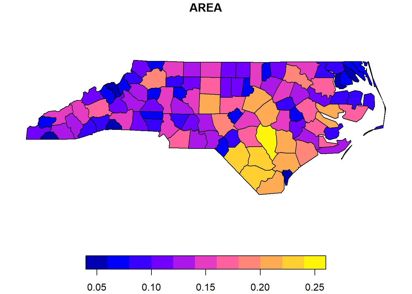
2 Raster data
Raster data (also referred to as grid data) is a spatial data structure that divides the region of study into rectangles of the same size called cells or pixels, and that can store one or more values for each of these cells (Figure 2.1). Raster data is used to represent spatially continuous phenomena, such as elevation, temperature or air pollution values.
In R, terra is the main package to work with raster data, which also has functionality to work with vector data. Before terra was developed, the raster package (Hijmans 2023) was used to analyze raster data. terra is very similar to raster but can do more and is faster. The stars package (Pebesma 2022b) can also be used to analyze raster data as well as spatial data cubes which are arrays with one or more spatial dimensions.
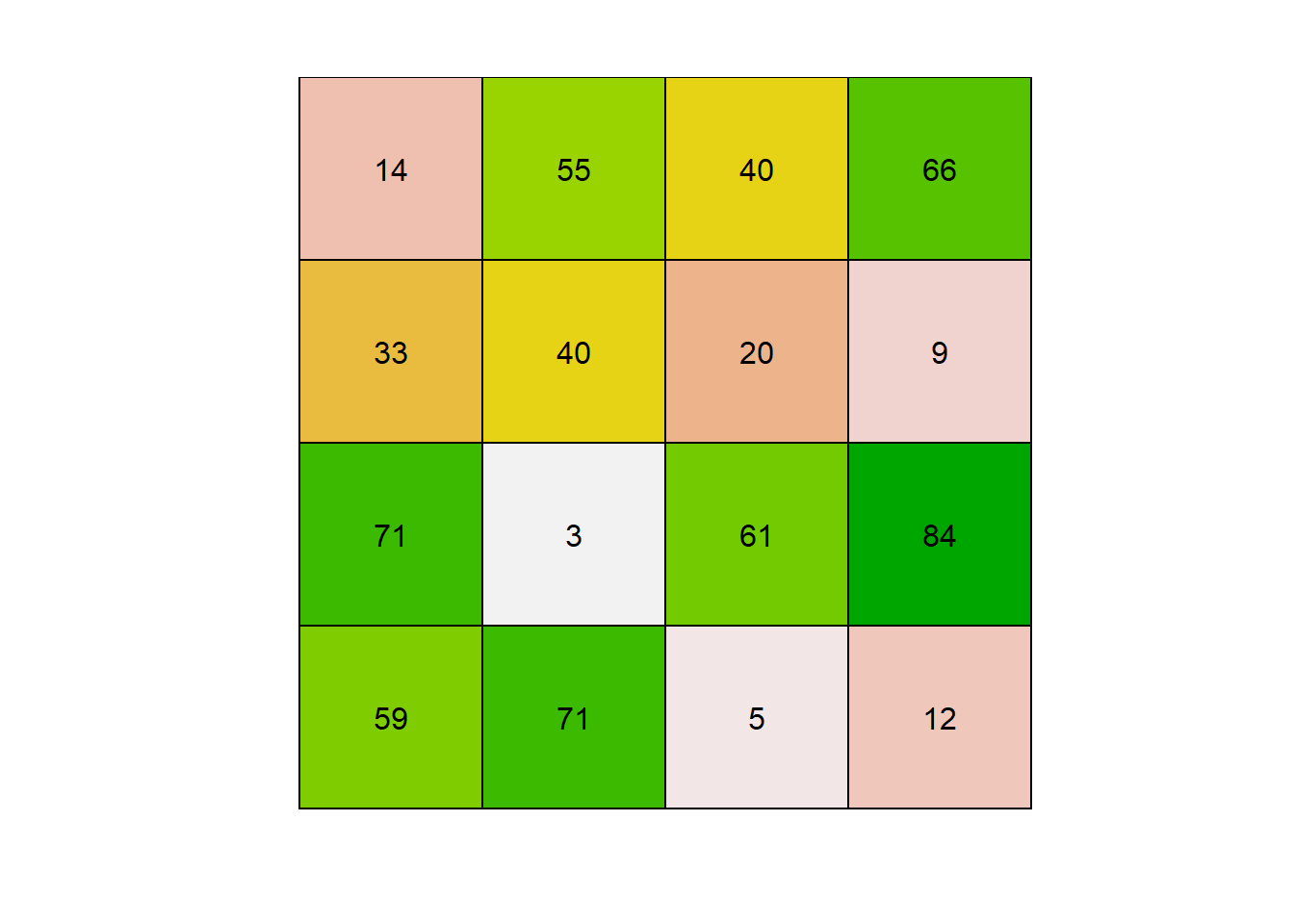
Figure 2.1: Example of raster data with cells colored according to their values.
2.1 GeoTIFF
Raster data often come in GeoTIFF format which has extension .tif.
Here, we use the terra::rast() function to read the elev.tif file of the terra package that represents elevation in Luxembourg.
library(terra)
pathraster <- system.file("ex/elev.tif", package = "terra")
r <- terra::rast(pathraster)
r
## class : SpatRaster
## dimensions : 90, 95, 1 (nrow, ncol, nlyr)
## resolution : 0.008333333, 0.008333333 (x, y)
## extent : 5.741667, 6.533333, 49.44167, 50.19167 (xmin, xmax, ymin, ymax)
## coord. ref. : lon/lat WGS 84 (EPSG:4326)
## source : elev.tif
## name : elevation
## min value : 141
## max value : 547plot(r)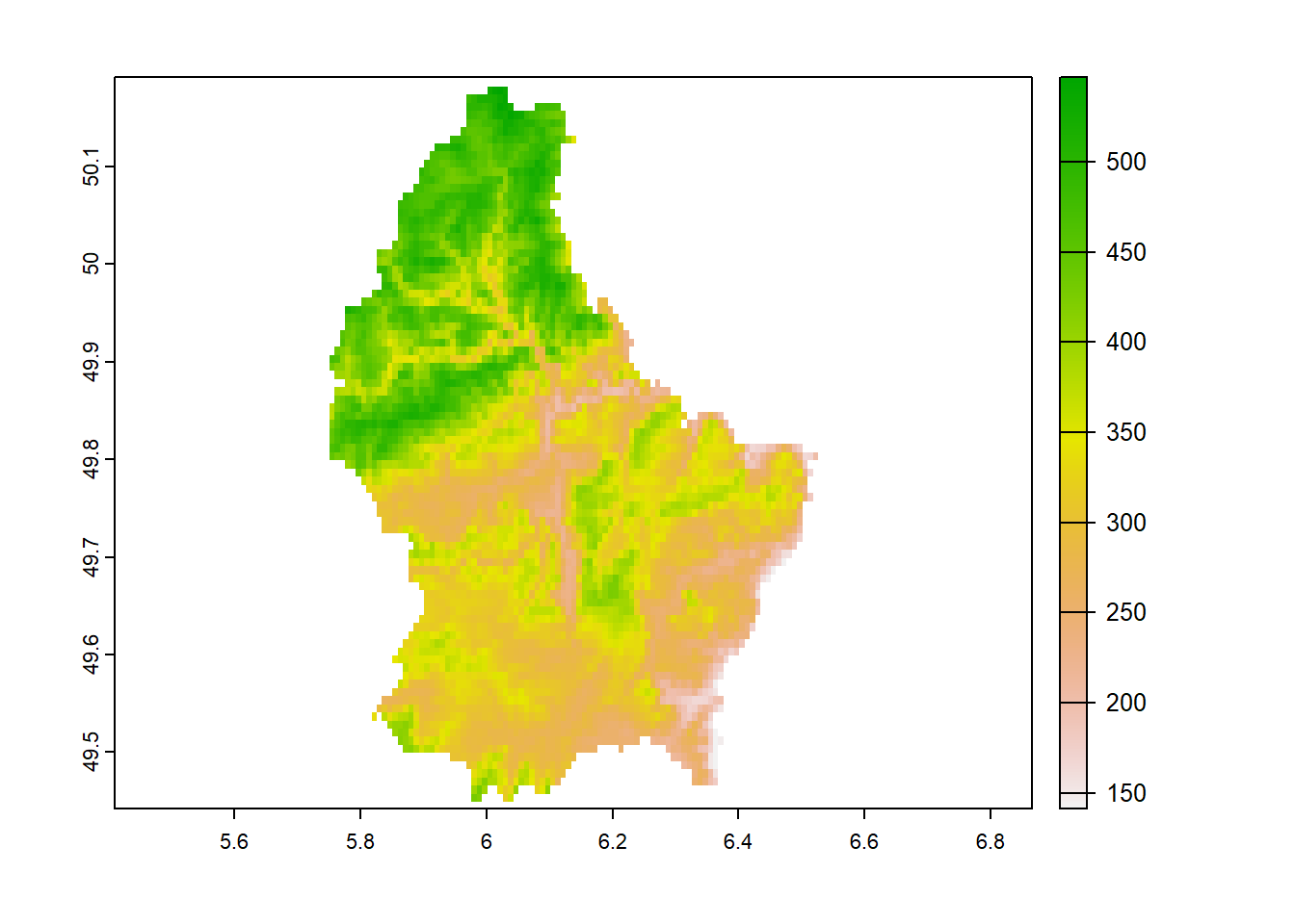
3 Coordinate Reference Systems (CRS)
The coordinate reference system (CRS) of spatial data specifies the origin and the unit of measurement of the spatial coordinates. CRSs are important for spatial data manipulation, analysis and visualization, and permit to deal with multiple data by transforming them to a common CRS. Locations on the Earth can be referenced using unprojected (also called geographic) or projected CRSs. The unprojected or geographic CRS uses latitude and longitude values to represent locations on the Earth’s three-dimensional ellipsoid surface. A projected CRS uses Cartesian coordinates to reference a location on a two-dimensional representation of the Earth.
3.1 Geographic CRS
In a geographic CRS, latitude and longitude values are used to identify locations on the Earth’s three-dimensional ellipsoid surface. Latitude values measure the angles north or south of the equator (0 degrees) and range from -90 degrees at the south pole to 90 degrees at the north pole. Longitude values measure the angles west or east of the prime meridian. Longitude values range from -180 degrees when running west to 180 degrees when running east (Figure 3.1).
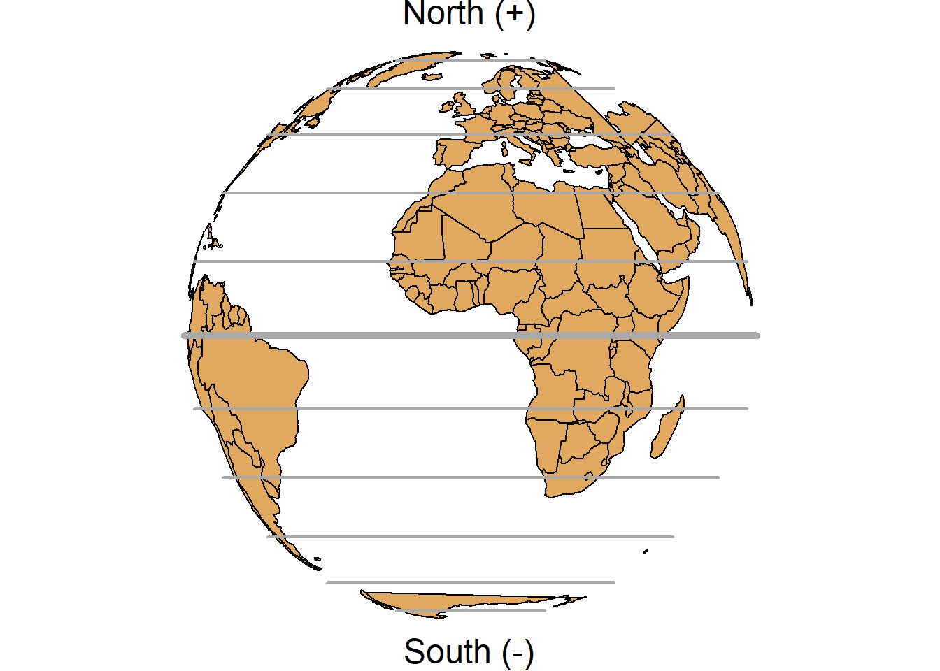
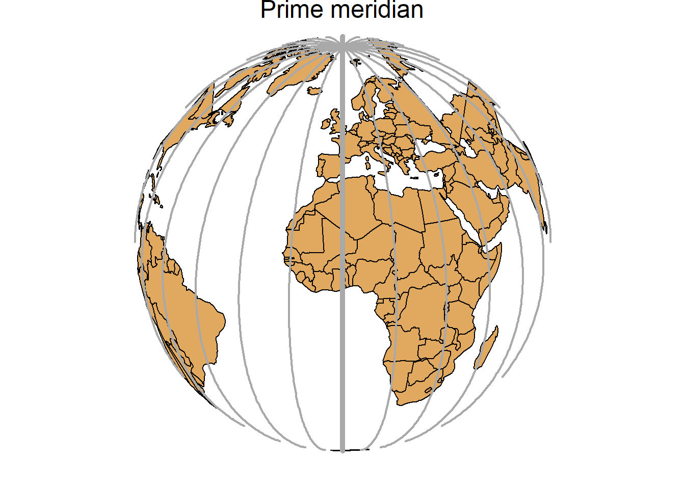
Figure 3.1: Parallels (left) and meridians (right).
Latitude and longitude coordinates may be expressed in degrees, minutes and seconds, or in decimal degrees. In decimal form, northern latitudes are positive and southern latitudes are negative. Also, eastern longitudes are positive and western longitudes are negative. For example, the location of New York City, USA, can be given by geographic coordinates as follows:
| Latitude | Longitude | |
|---|---|---|
| Degrees, Minutes and Seconds | 40\(^o\) 43’ 50.1960’’ North | 73\(^o\) 56’ 6.8712’’ West |
| Decimal degrees (North/South and West/East) | 40.730610\(^o\) North | 73.935242\(^o\) West |
| Decimal degrees (Positive/Negative) | 40.730610 | -73.935242 |
3.2 Projected CRS
Projected CRSs use Cartesian coordinates to reference a location on a two-dimensional representation of the Earth. All projections produce distortion of the Earth’s surface in some fashion, and cannot simultaneously preserve all area, direction, shape and distance properties. For example, Figure 3.2 shows world maps using two different projections, namely, Mercator and Robinson projections.
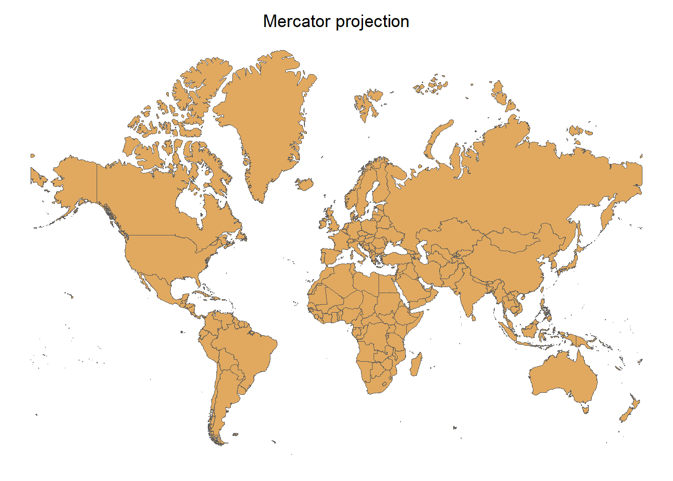
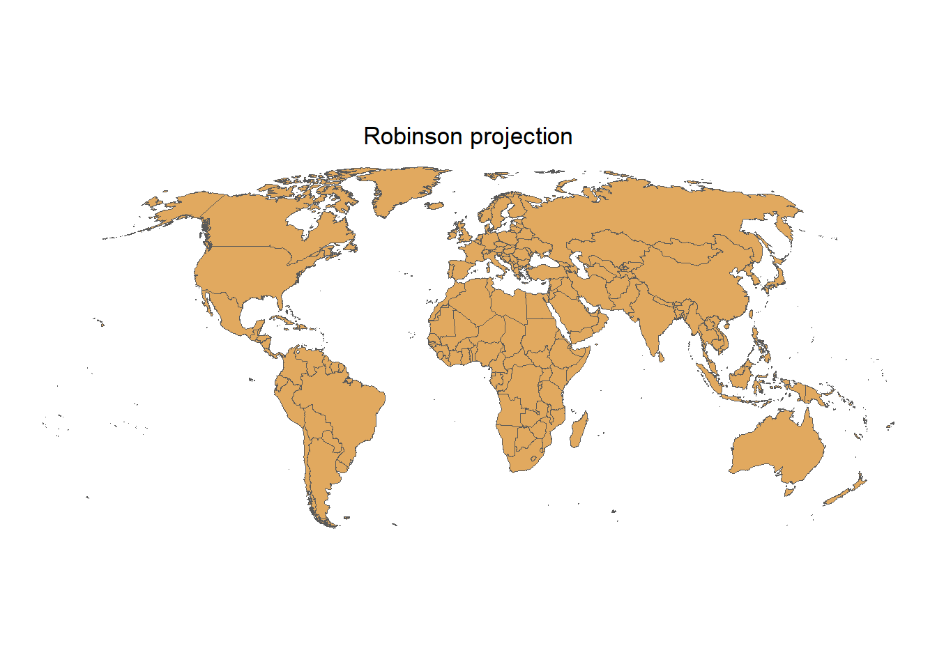
Figure 3.2: World maps with Mercator (left) and Robinson (right) projections.
A common projection is the Universal Transverse Mercator (UTM) projection. This projection is conformal meaning that it preserves angles and therefore shapes across small regions. However, it distorts distances and areas. In the UTM projection, a location is given by the zone number (60 zones), hemisphere (north or south), and Easting and Northing coordinates in the zone in meters. Eastings and Northings are referenced from the central meridian and equator, respectively, of each zone.
3.3 EPSG codes
Most common CRSs can be specified by providing their EPSG (European Petroleum Survey Group) codes or their Proj4 strings.
Common spatial projections can be found at https://spatialreference.org/ref/.
Details of a given projection can be inspected using the st_crs() function of the sf package.
For example, the EPSG code 4326 refers to the WGS84 longitude/latitude projection.
st_crs("EPSG:4326")$Name## [1] "WGS 84"st_crs("EPSG:4326")$proj4string## [1] "+proj=longlat +datum=WGS84 +no_defs"st_crs("EPSG:4326")$epsg## [1] 43263.4 Transforming CRS with sf and terra
Functions sf::st_crs() and terra::crs() allow us to get the CRS of spatial data.
These functions also allow us to set a CRS to spatial data by using
st_crs(x) <- value if x is an sf object, and crs(r) <- value if r is a raster.
Notice that setting a CRS does not transform the data, it just changes the CRS label.
We may want to set a CRS to data that does not come with CRS, and the CRS should be what it is, not what we would like it to be. We use sf::st_transform() and terra::project() to transform the sf or raster data, respectively, to a new CRS.
For sf data, we can read and get the CRS, and transform the data to a new CRS as follows:
library(sf)
pathshp <- system.file("shape/nc.shp", package = "sf")
map <- st_read(pathshp, quiet = TRUE)
# Get CRS
# st_crs(map)
# Transform CRS
map2 <- st_transform(map, crs = "EPSG:4326")
# Get CRS
# st_crs(map2)
We can use terra to read and get the CRS, and transform the data to a new CRS of a raster as follows:
library(terra)
pathraster <- system.file("ex/elev.tif", package = "terra")
r <- rast(pathraster)
# Get CRS
# crs(r)
# Transform CRS
r2 <- terra::project(r, "EPSG:2169")
# Get CRS
# crs(r2)
Alternatively, as we may want transformed data that exactly lines up with other raster data we are using, we can project using an existing raster with the geometry we wish. For example,
# x is existing raster
# r is raster we project
r2 <- terra::project(r, x)
4 Old spatial packages
Before the sf package was developed, the sp package was used to represent and work with vector spatial data.
sp as well as the rgdal (Bivand, Keitt, and Rowlingson 2023), rgeos (Bivand and Rundel 2022) and maptools (Bivand and Lewin-Koh 2022) packages are not longer maintained and will retire.
Using old packages, the rgdal::readOGR() function can be used to read a file.
Data can be accessed with sp_object@data,
and the sp::spplot() function can be used to plot sp spatial objects.
library(sf)
library(sp)
library(rgdal)
pathshp <- system.file("shape/nc.shp", package = "sf")
sp_object <- rgdal::readOGR(pathshp, verbose = FALSE)
class(sp_object)
## [1] "SpatialPolygonsDataFrame"
## attr(,"package")
## [1] "sp"# sp::spplot(sp_object, zcol = "BIR74")The st_as_sf() function of sf can be used to transform an sp object to an sf object (st_as_sf(sp_object)).
Also, an sf object can be transformed to an sp object with as(sf_object, "Spatial").