The terra package for raster and vector data
Paula Moraga, KAUST
Materials based on the book Geospatial Health Data (2019, Chapman & Hall/CRC)
http://www.paulamoraga.com/book-geospatial
The terra package (Hijmans 2022) has functions to create, read, manipulate, and write raster and vector data.
Raster data is commonly used to represent spatially continuous phenomena by dividing the study region into a grid of equally sized rectangles (referred to as cells or pixels) with the values of the variable of interest.
In terra, multilayer raster data is represented with the SpatRaster class.
The SpatVector class is used to represent vector data such as points, lines and polygons, and their attributes.
In this chapter, we provide examples on how to read, create, and operate with raster and vector data using terra.
1 Raster data
The rast() function can be used to create and read raster data.
The writeRaster() function allows us to write raster data.
For example, here we use rast() to read raster data representing elevation in Luxembourg from a file from the terra package, and assign it to an object r of class SpatRaster (Figure 1.1).
library(terra)
pathraster <- system.file("ex/elev.tif", package = "terra")
r <- rast(pathraster)
plot(r)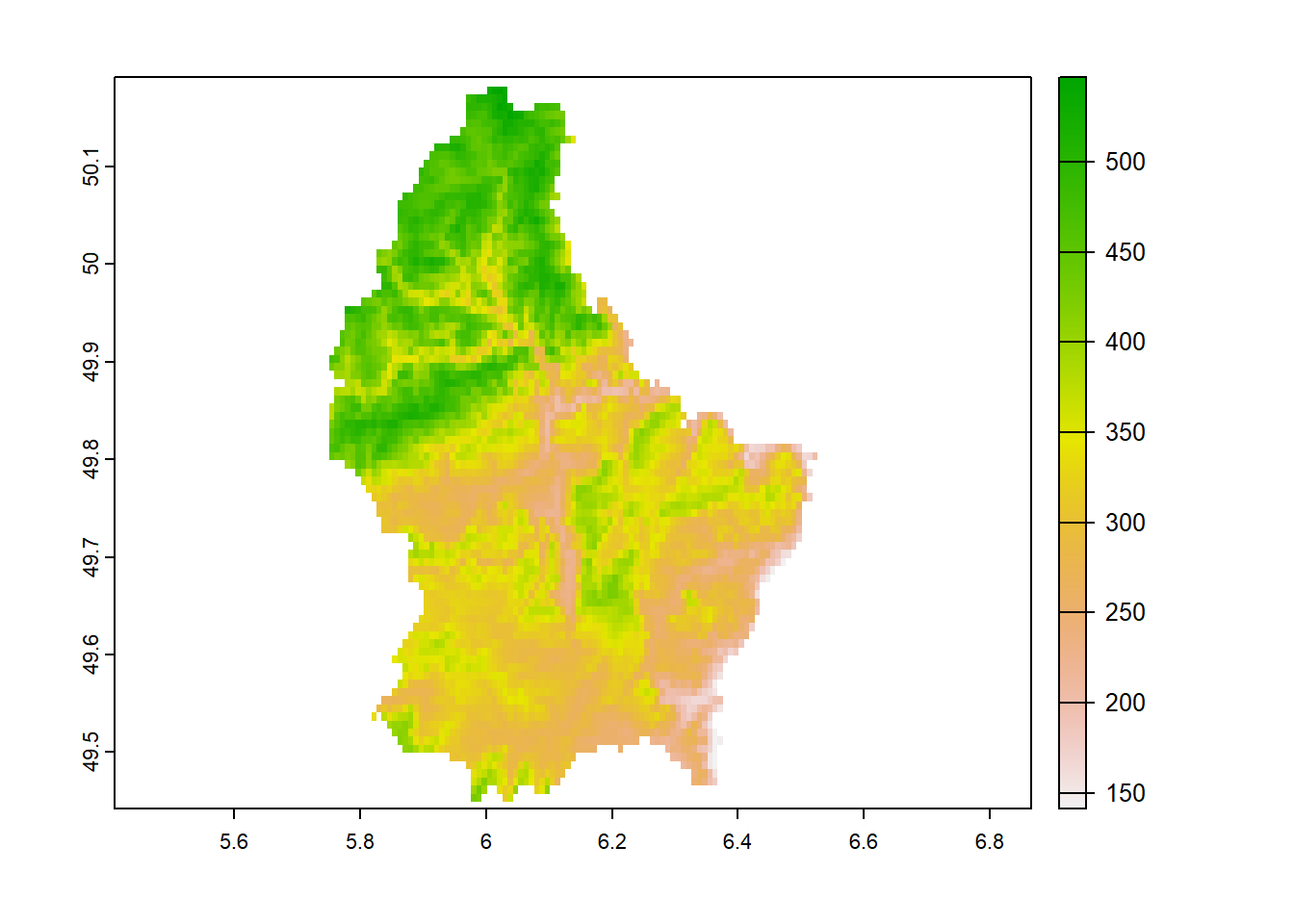
Figure 1.1: Elevation raster in Luxembourg obtained from terra.
We can also use rast() to create a SpatRaster object r by specifying the number of columns, the number of rows, as well as the minimum and maximum x and y values.
r <- rast(ncol = 10, nrow = 10,
          xmin = -150, xmax = -80, ymin = 20, ymax = 60)
r
## class : SpatRaster
## dimensions : 10, 10, 1 (nrow, ncol, nlyr)
## resolution : 7, 4 (x, y)
## extent : -150, -80, 20, 60 (xmin, xmax, ymin, ymax)
## coord. ref. : lon/lat WGS 84We can get the size of the raster with several functions.
nrow(r) # number of rows
ncol(r) # number of columns
dim(r) # dimension
ncell(r) # number of cells
We use values() to set and access values of the raster.
Figure 1.2 shows the values corresponding to each of the cells of the raster created.
values(r) <- 1:ncell(r)
plot(r)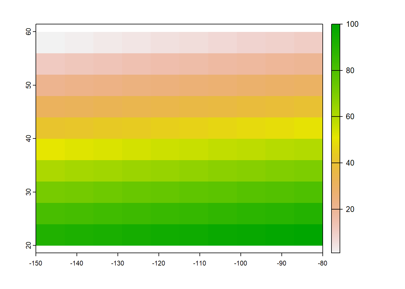
Figure 1.2: Raster and values corresponding to each of the cells created with terra.
We can also create a multilayer object using c().
r2 <- r * r
s <- c(r, r2)
Layers can be subsetted with [[ ]].
plot(s[[2]]) # layer 2Many generic functions can be used to operate with rasters as shown in the following examples.
plot(min(s))
plot(r + r + 10)
plot(round(r))
plot(r == 1)
2 Vector data
The class SpatVector of terra allows us to represent vector data such as points, lines, and polygons, as well as the attributes that describe these geometries. We can use vect() to read a shapefile, and writeVector() to write a SpatVector to a file.
Here, we obtain the map with the divisions of Luxembourg that is in the shapefile file lux.shp of terra.
pathshp <- system.file("ex/lux.shp", package = "terra")
v <- vect(pathshp)
We can also use the vect() function to create a SpatVector. For example, here we create a SpatVector that contains longitude and latitude coordinates of point locations, and attributes representing character names and numeric values for each of the points.
# Longitude and latitude values
long <- c(-0.118092, 2.349014, -3.703339, 12.496366)
lat <- c(51.509865, 48.864716, 40.416729, 41.902782)
longlat <- cbind(long, lat)

# CRS
crspoints <- "+proj=longlat +datum=WGS84"

# Attributes for points
d <- data.frame(
place = c("London", "Paris", "Madrid", "Rome"),
value = c(200, 300, 400, 500))

# SpatVector object
pts <- vect(longlat, atts = d, crs = crspoints)

# pts
# plot(pts)
3 Cropping, masking and aggregating raster data
The terra package provides several functions to work with raster data. Here, we show examples on how to crop, mask and aggregate raster data by using a raster file representing temperature data.
First, we use the worldclim_country() function of the geodata package (Hijmans, Ghosh, and Mandel 2022) to download global temperature data from the WorldClim database.
Specifically, we download monthly average temperature in degree Celsius by specifying the country ("Spain"), the variable mean temperature var = "tavg", the resolution res = 10, and the path where to download the data to as a temporary file path = tempdir().
Figure 3.1 shows maps of the monthly average temperature in Spain.
library(terra)
r <- geodata::worldclim_country(country = "Spain", var = "tavg",
                                res = 10, path = tempdir())
plot(r)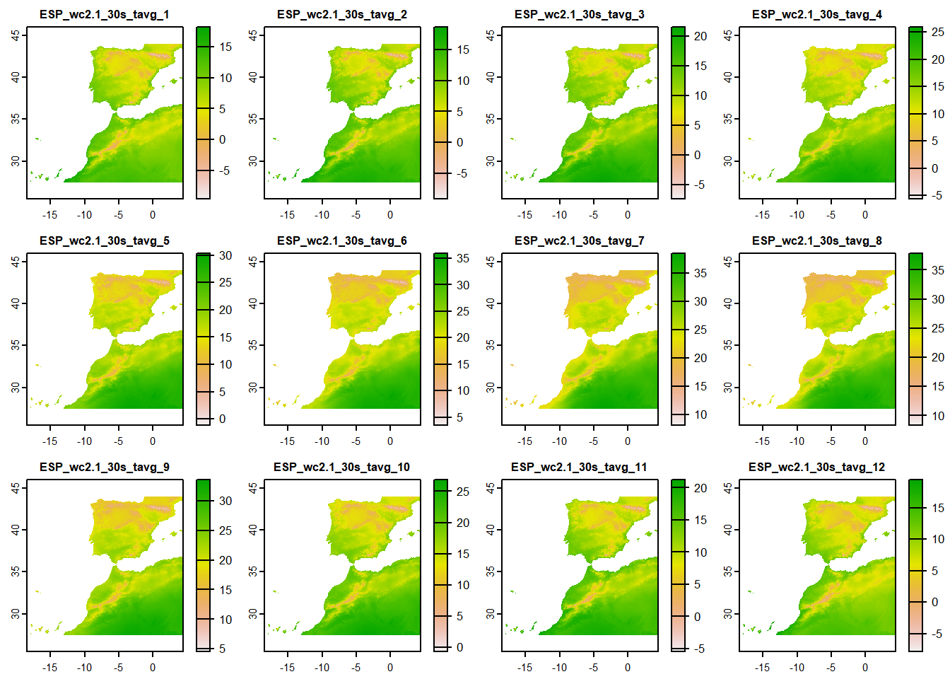
Figure 3.1: Monthly average temperature in Spain obtained from geodata.
We can average the temperature raster data over months with the mean() function (Figure 3.2).
r <- mean(r)
plot(r)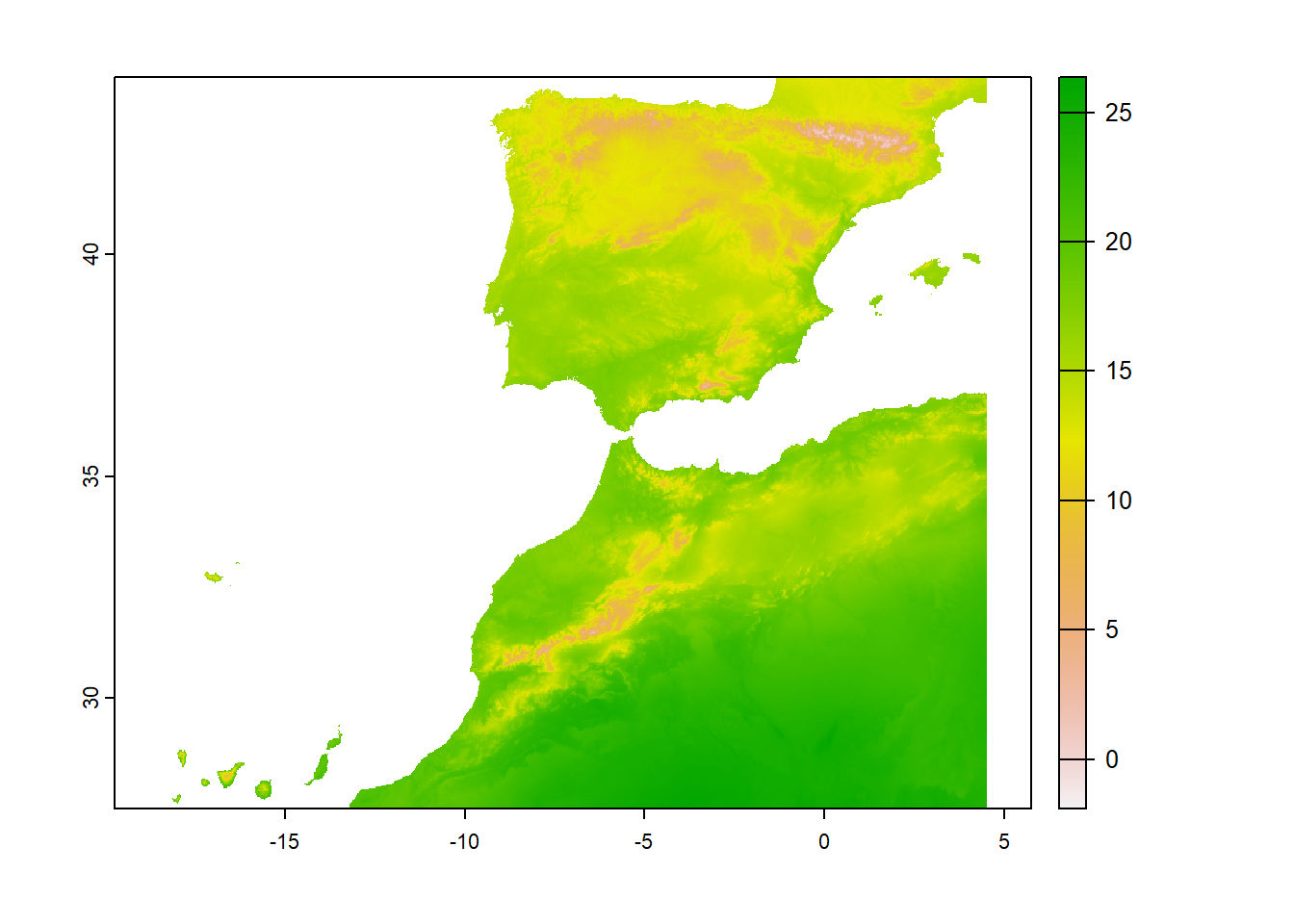
Figure 3.2: Raster representing the average annual temperature in Spain.
We also download the map of Spain with the rnaturalearth package (South 2017), and delete the Canary Islands region (Figure 3.3).
library(ggplot2)
map <- rnaturalearth::ne_states("Spain", returnclass = "sf")
map <- map[-which(map$region == "Canary Is."), ] # delete region
ggplot(map) + geom_sf()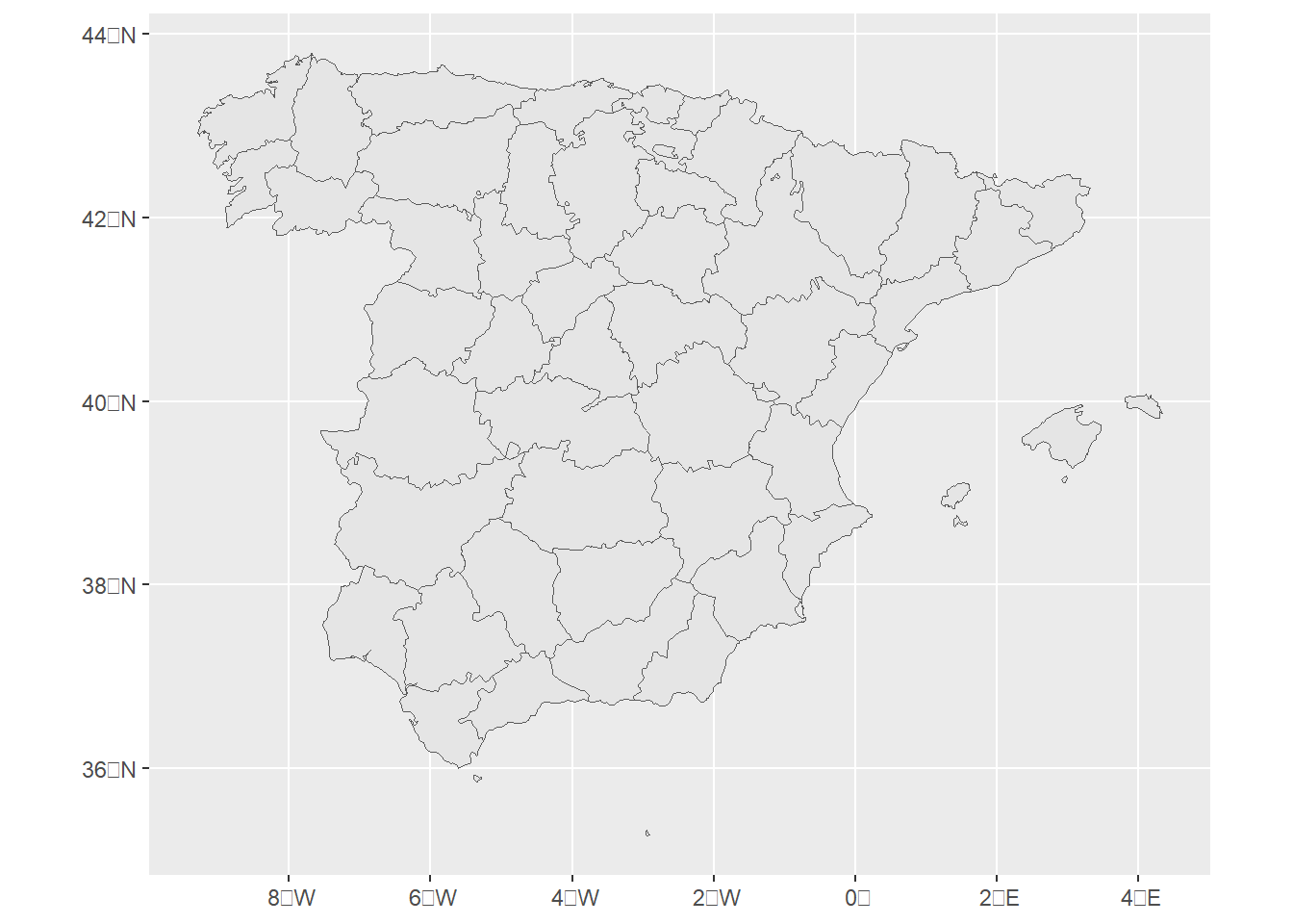
Figure 3.3: Map of Spain excluding the Canary Islands region obtained from rnaturalearth.
We obtain the spatial extent of the map with terra:ext().
sextent <- terra::ext(map)Then, we can use crop() to remove the part of the raster that is outside the spatial extent (Figure 3.4).
r <- terra::crop(r, sextent)
plot(r)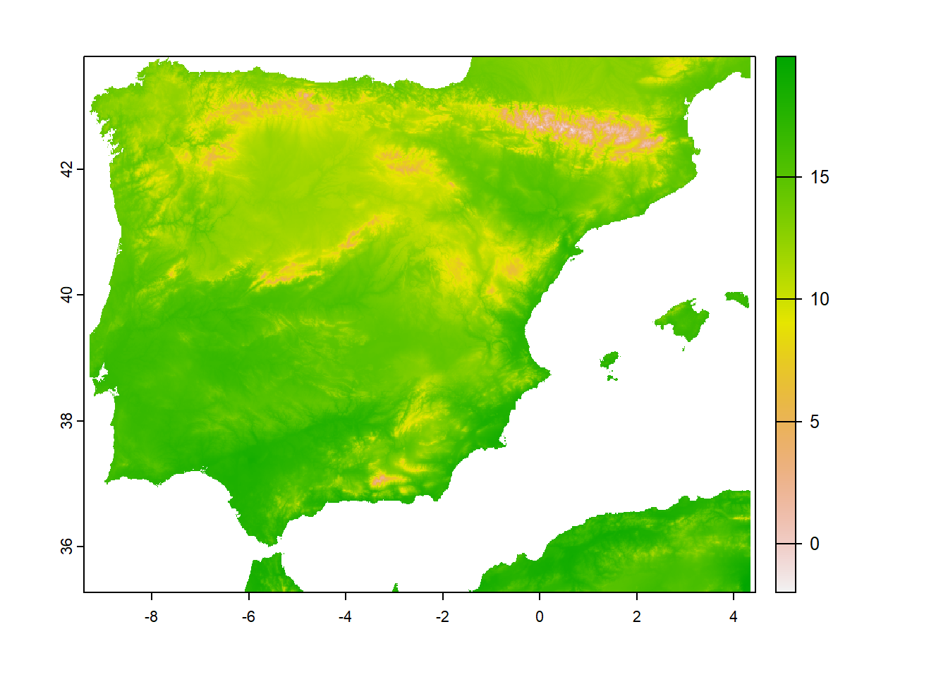
Figure 3.4: Cropped raster representing the average annual temperature in Spain.
We can use the mask() function to convert all values outside the map to NA (Figure 3.5).
r <- terra::mask(r, vect(map))
plot(r)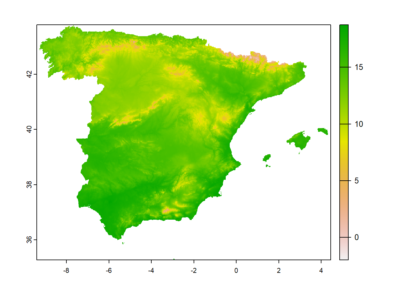
Figure 3.5: Masked raster representing the average annual temperature in Spain.
The aggregate() function of terra can be used
to aggregate groups of cells of a raster in order to create a new raster with a lower resolution (i.e., larger cells).
The argument fact of aggregate() denotes the aggregation factor expressed as number of cells in each direction (horizontally and vertically), or two integers denoting the horizontal and vertical aggregation factor. Argument fun specifies the function used to aggregate values (e.g., mean).
Figure 3.6 shows a low resolution raster of average annual temperatures in Spain obtained using the aggregate() function.
r <- terra::aggregate(r, fact = 20, fun = "mean", na.rm = TRUE)
plot(r)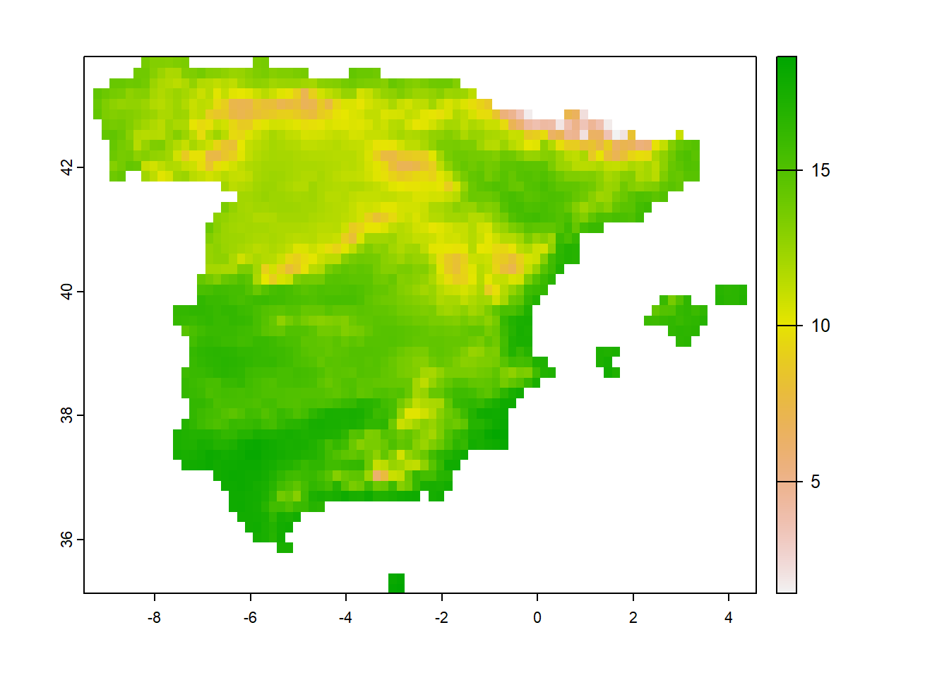
Figure 3.6: Low resolution raster representing the average annual temperature in Spain.
4 Extracting raster values at points
Given a raster of class SpatRaster, we can extract the raster values at a set of points with the extract() function of terra. Here, we provide an example of the use of extract() using a raster representing the elevation of Luxembourg, and a vector file with the divisions of Luxembourg from files in the terra package.
library(terra)
# Raster (SpatRaster)
r <- rast(system.file("ex/elev.tif", package = "terra"))
# Polygons (SpatVector)
v <- vect(system.file("ex/lux.shp", package = "terra"))
We use the terra functions centroids() to obtain the centroids of the division polygons, and crds() to obtain their coordinates.
points <- crds(centroids(v))Figure 4.1 shows the elevation raster, the polygons, and the points of the centroid locations.
plot(r)
plot(v, add = TRUE)
points(points)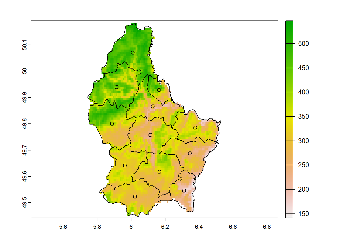
Figure 4.1: Elevation raster, and division and centroids of polygons in Luxembourg.
Now, we obtain the values of the raster at points using extract() passing as first argument the SpatVector object with the raster, and as second argument a data frame with the points.
# data frame with the coordinates
points <- as.data.frame(points)
valuesatpoints <- extract(r, points)
cbind(points, valuesatpoints)
5 Extracting and averaging raster values within polygons
We can also use extract() to obtain the values of raster objects of class SpatRaster within polygons of class SpatVector.
By default, cells extracted within each polygon are cells that have centers covered by the polygon. We can set the argument weights = TRUE to get, apart from the cell values, the percentage of each cell covered by the polygon and this can be used to compute area-weighted averages.
The argument fun of extract() can be used to specify a function (e.g., mean) that summarizes the extracted values by polygon.
# Extracted raster cells within each polygon
head(extract(r, v, na.rm = TRUE))
# Extracted raster cells and percentage of area
# covered within each polygon
head(extract(r, v, na.rm = TRUE, weights = TRUE))Thus, the average raster values by polygon are obtained with extract() as follows.
# Average raster values by polygon
v$avg <- extract(r, v, mean, na.rm = TRUE)$elevation
The area-weighted average raster values by polygon are obtained with extract() setting weights = TRUE.
# Area-weighted average raster values by polygon (weights = TRUE)
v$weightedavg <- extract(r, v, mean, na.rm = TRUE,
                 weights = TRUE)$elevation
Figure 5.1 shows maps of the elevation averages and area-weighted averages in each of the Luxembourg divisions created with the ggplot2 and tidyterra packages.
library(ggplot2)
library(tidyterra)

# Plot average raster values within polygons
ggplot(data = v) + geom_spatvector(aes(fill = avg)) +
  scale_fill_terrain_c()
# Plot area-weighted average raster values within polygons
ggplot(data = v) + geom_spatvector(aes(fill = weightedavg)) +
  scale_fill_terrain_c()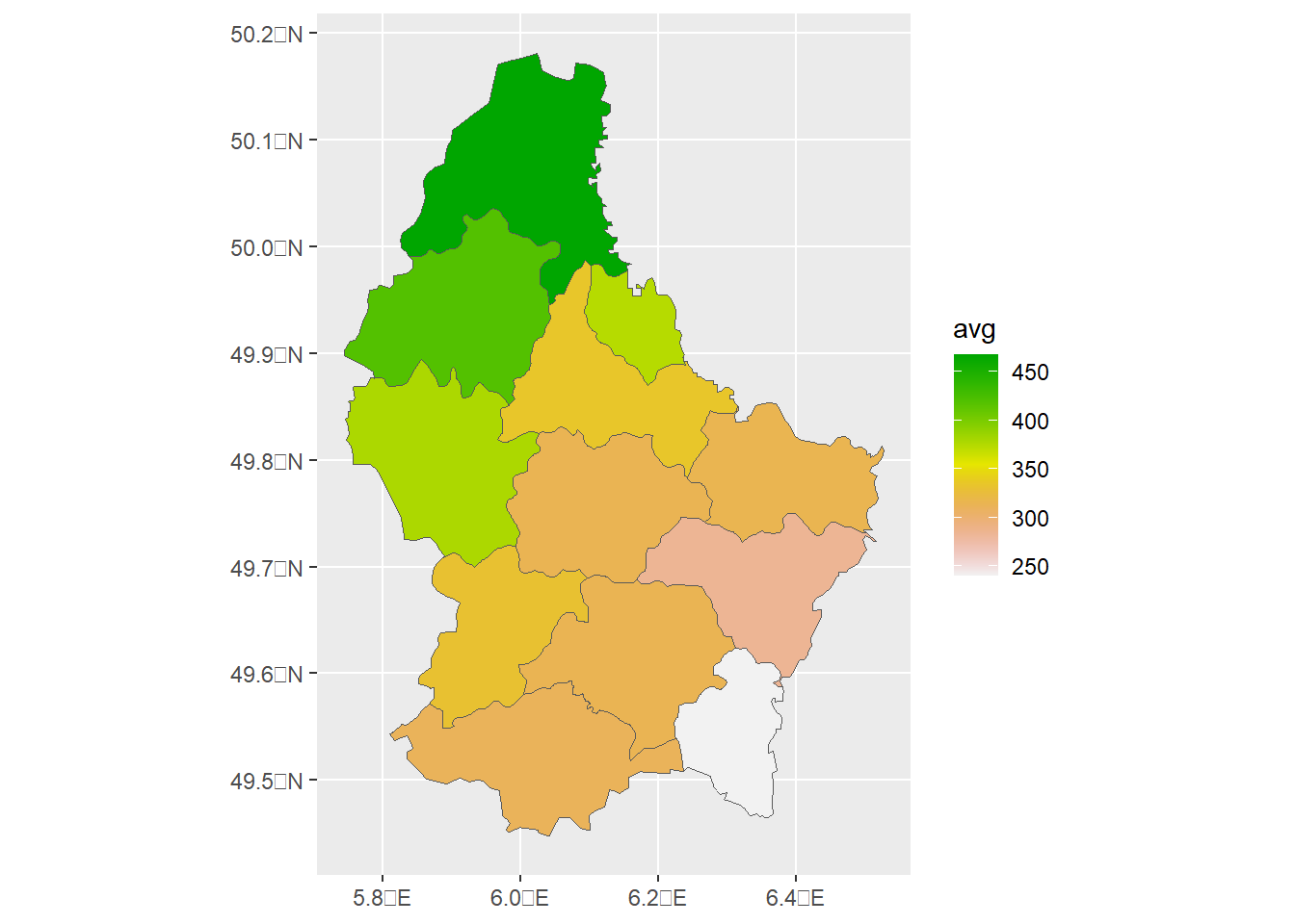
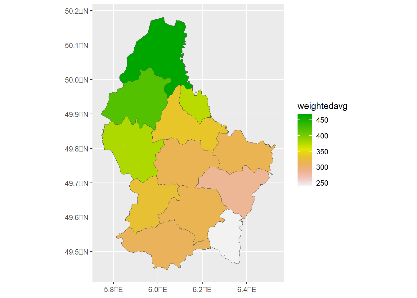
Figure 5.1: Average and area-weighted average of elevation values in each of the divisions of Luxembourg.