Risk assessment of travel-related spread of disease with epiflows

epiflows

outbreaks

epidemics

In this post I show how to use the R package epiflows for risk assessment of travel-related spread of disease. Infectious diseases can spread beyond national borders. Residents of an infectious location can travel abroad and infect people living there. Also, travelers can acquire a disease while staying in a foreign country, and then seed new outbreaks in their home country after their return. The amount of disease spread will depend on factors such as the number of infected cases, population flows between locations, lengths of stay, and disease incubation and infectious periods. The epiflows package uses the mathematical model developed by Dorigatti et al. (2017) to integrate all these factors and calculate the mean number of infections that could be spread to other locations together with uncertainty measures. Here, I explain how to use epiflows to estimate the spread of yellow fever from Espirito Santo, Brazil, to other countries in the period December 2016 to May 2017. Details of the underlying model and other options of the package can be seen in Moraga et al. (2018).

Data

We use the data of yellow fever in Brazil that is contained in the epiflows package as data("Brazil_epiflows"). This data contains an object of class epiflows which has, for each location, the population, the number of disease cases, dates, and lengths of stay. Brazil_epiflows also contains the population flows between the Brazil states and other countries.

library(epiflows)
data("Brazil_epiflows")
Brazil_epiflows


/// Epidemiological Flows //

  // class: epiflows, epicontacts
  // 15 locations; 100 flows; directed
  // optional variables: pop_size, duration_stay, num_cases, first_date, last_date 

  // locations

# A tibble: 15 × 6
   id                 location_population num_cases_time_window first_date_cases
   <chr>                            <dbl>                 <dbl> <fct>           
 1 Espirito Santo                 3973697                  2600 2017-01-04      
 2 Minas Gerais                  20997560                  4870 2016-12-19      
 3 Rio de Janeiro                16635996                   170 2017-02-19      
 4 Sao Paulo                     44749699                   200 2016-12-17      
 5 Southeast Brazil              86356952                  7840 2016-12-17      
 6 Argentina                           NA                    NA <NA>            
 7 Chile                               NA                    NA <NA>            
 8 Germany                             NA                    NA <NA>            
 9 Italy                               NA                    NA <NA>            
10 Paraguay                            NA                    NA <NA>            
11 Portugal                            NA                    NA <NA>            
12 Spain                               NA                    NA <NA>            
13 United Kingdom                      NA                    NA <NA>            
14 United States of …                  NA                    NA <NA>            
15 Uruguay                             NA                    NA <NA>            
# ℹ 2 more variables: last_date_cases <fct>, length_of_stay <dbl>

  // flows

# A tibble: 100 × 3
   from             to         n
   <chr>            <chr>  <dbl>
 1 Espirito Santo   Italy  2828.
 2 Minas Gerais     Italy 15714.
 3 Rio de Janeiro   Italy  8164.
 4 Sao Paulo        Italy 34039.
 5 Southeast Brazil Italy 76282.
 6 Espirito Santo   Spain  3270.
 7 Minas Gerais     Spain 18176.
 8 Rio de Janeiro   Spain  9443.
 9 Sao Paulo        Spain 39371.
10 Southeast Brazil Spain 88231.
# ℹ 90 more rows

Call estimate_risk_spread()

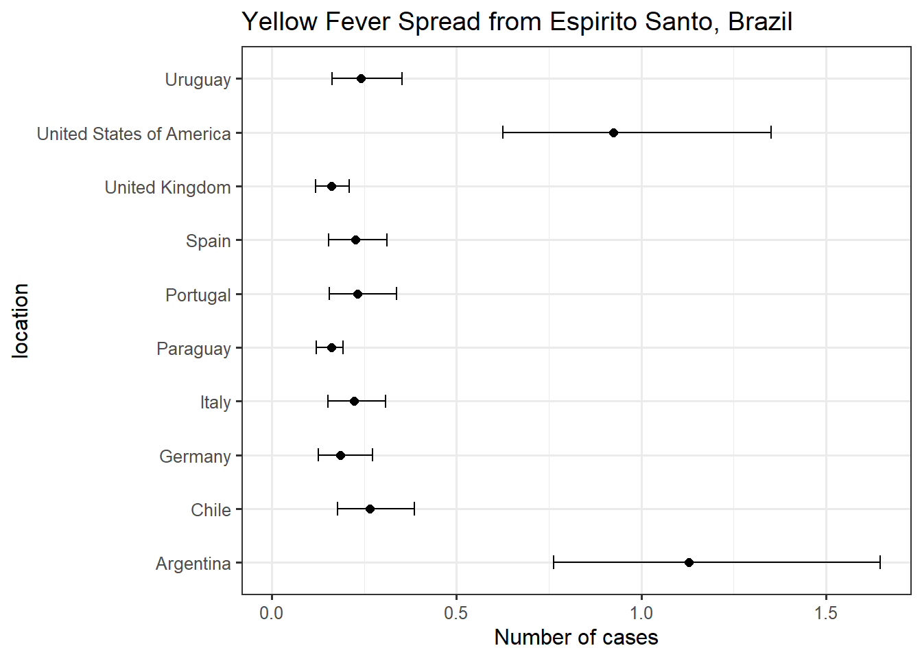
We can use the function estimate_risk_spread() to calculate the mean number of cases spread from the state Espirito Santo to other locations and the 95% confidence intervals. To call this function we need to specify the epiflows object (Brazil_epiflows), the code of the location ("Espirito Santo"), the functions of the disease incubation and infectious distributions, and the number of simulations.

set.seed(2018-07-25)
res <- estimate_risk_spread(Brazil_epiflows, 
                            location_code = "Espirito Santo",
                            r_incubation = function(n) rlnorm(n, 1.46, 0.35),
                            r_infectious = function(n) rnorm(n, 4.5, 1.5/1.96),
                            n_sim = 100000
                           )
res

                         mean_cases lower_limit_95CI upper_limit_95CI
Italy                     0.2233656        0.1520966        0.3078136
Spain                     0.2255171        0.1537452        0.3126801
Portugal                  0.2317019        0.1565528        0.3383112
Germany                   0.1864162        0.1259548        0.2721890
United Kingdom            0.1613418        0.1195261        0.2089475
United States of America  0.9253419        0.6252207        1.3511047
Argentina                 1.1283506        0.7623865        1.6475205
Chile                     0.2648277        0.1789370        0.3866836
Uruguay                   0.2408942        0.1627681        0.3517426
Paraguay                  0.1619724        0.1213114        0.1926966

Results

The results object is a data frame containing the mean number of cases spread to each country and the lower and upper limits of the 95% confidence intervals. We can plot the results with the function ggplot() of the ggplot2 package as follows.

library(ggplot2)
res$location <- rownames(res)
ggplot(res, aes(x = mean_cases, y = location)) +
  geom_point(size = 2) +
  geom_errorbarh(aes(xmin = lower_limit_95CI, xmax = upper_limit_95CI), height = .25) +
  theme_bw(base_size = 12, base_family = "Helvetica") +
  ggtitle("Yellow Fever Spread from Espirito Santo, Brazil") +
  xlab("Number of cases") +
  xlim(c(0, NA))

Visualization of population flows

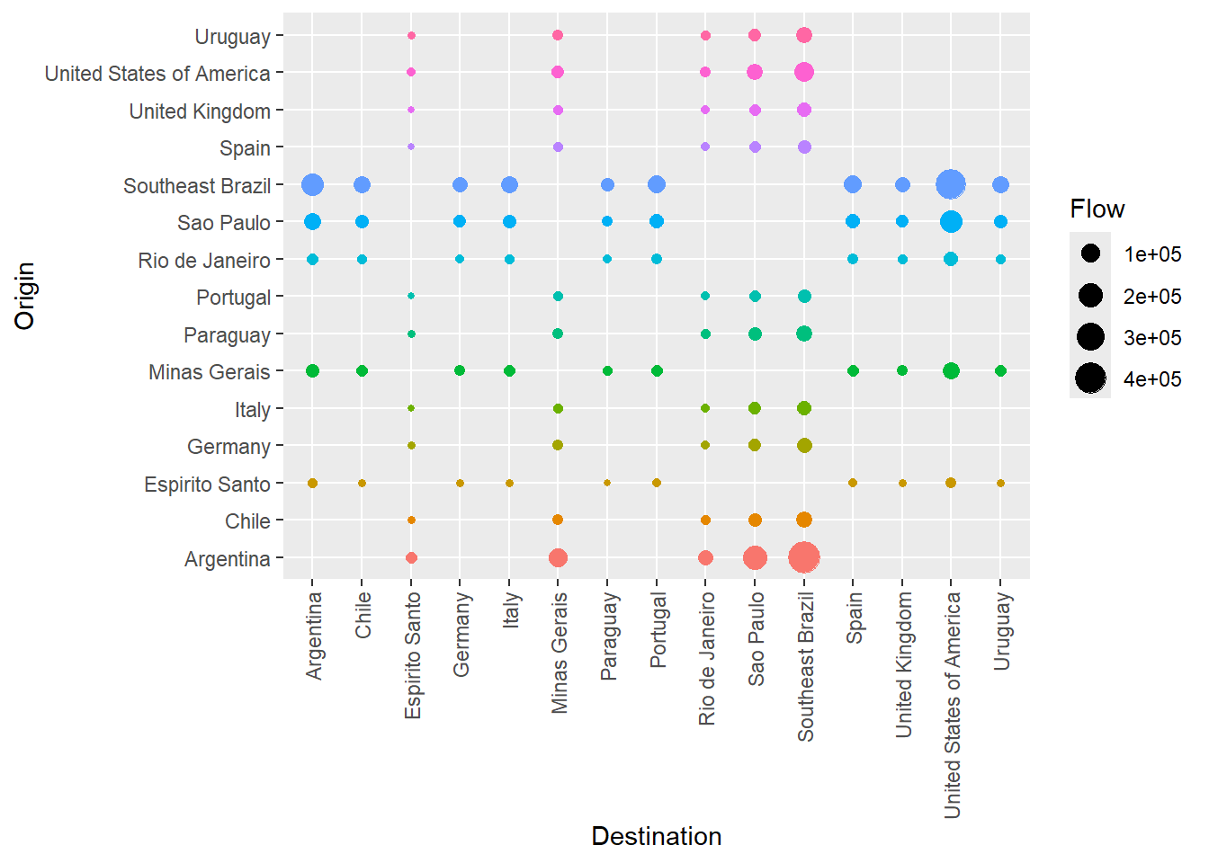
epiflows also incorporates functions to plot population flows between locations. There are three types of plots that can be produced:

Interactive map. This type of plot requires Brazil_epiflows to contain the coordinates of the locations. In this example the coordinates are in data frame YF_coordinates and can be added to Brazil_epiflows with the add_coordinates() function of epiflows.

data("YF_coordinates")
Brazil_epiflows <- add_coordinates(Brazil_epiflows, coordinates = YF_coordinates[, -1])

plot(Brazil_epiflows, type = "map")

Dynamic network with locations shown as nodes and connections between them representing population flows.

plot(Brazil_epiflows, type = "network")

Grid with population flows shown as points.

plot(Brazil_epiflows, type = "grid")

Conclusion

The epiflows package allows the identification of locations where diseases are most likely to spread. This information can help public health officials to limit the global spread of local outbreaks.

epiflows has been developed by several members of the R Epidemics Consortium (RECON). You can see the development version here. Please get in touch via GitHub issues if you have any comment, question or would like to contribute!

References

Moraga P, Dorigatti I, Kamvar ZN, Piatkowski P, Toikkanen SE, Nagraj VP, Donnelly CA and Jombart T. (2018), epiflows: an R package for risk assessment of travel-related spread of disease. F1000Research, 7:1374.

Dorigatti I, Hamlet A, Aguas R, Cattarino L, Cori A, Donnelly CA, Garske T, Imai N and Ferguson NM (2017), International risk of yellow fever spread from the ongoing outbreak in Brazil, December 2016 to May 2017. Euro Surveill. 22(28):pii=30572.