13 Introduction to Shiny

Shiny (Chang et al. 2023) is a web application framework for R that enables to build interactive web applications. Shiny apps are useful to communicate information as interactive data explorations instead of static documents. A Shiny app is composed of a user interface ui which controls the layout and appearance of the app, and a server() function which contains the instructions to build the objects displayed in the user interface. Shiny apps permit user interaction by means of a functionality called reactivity. In this way, elements in the app are updated whenever users modify some options. This permits a better exploration of the data and greatly facilitates communication with other researchers and stakeholders. To create Shiny apps, there is no web development experience required, although greater flexibility and customization can be achieved by using HTML, CSS or JavaScript.

This chapter explains the basic principles to build a Shiny app. It shows how to build the user interface and server parts of an app, and how to create reactivity. It also shows how to design a basic layout for the user interface, and explains the options for sharing the app with others. More advanced topics such as customization of reactions and appearance of the app can be found in the Shiny tutorials website. Examples of more advanced Shiny apps can be seen in the Shiny gallery. Chapter 14 explains how to create interactive dashboards with Shiny, and Chapter 15 contains a step-by-step description to build a Shiny app that permits to upload and visualize spatio-temporal data.

13.1 Examples of Shiny apps

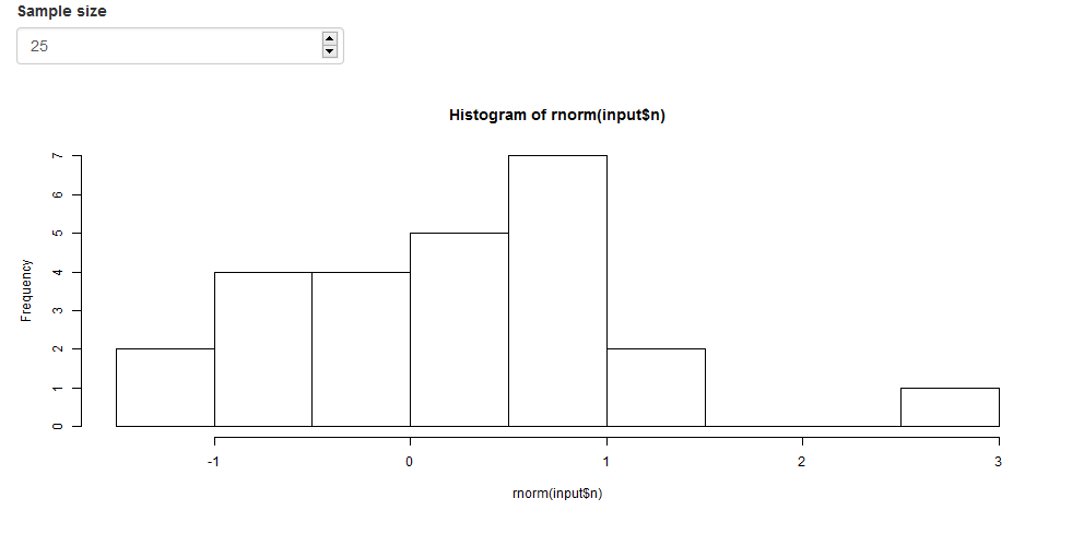
FIGURE 13.1: Snapshot of the first Shiny app.

An example of a Shiny app is shown in Figure 13.1. This app contains a numeric box where we can introduce a number, and a histogram that is built with values that are randomly generated from a normal distribution. The number of values used to build the histogram is given by the number specified in the numeric box. Each time we introduce a different number in the numeric box, the histogram is rebuilt with new generated values.

Figure 13.2 shows a second Shiny app. This app shows a barplot with the number of telephones in a given world region across several years. The region can be selected from a dropdown menu that contains all the possible regions. The barplot is rebuilt each time a different region is selected.

FIGURE 13.2: Snapshot of the second Shiny app.

13.2 Structure of a Shiny app

A Shiny app can be built by creating a directory (called, for example, appdir) that contains an R file (called, for example, app.R) with three components:

a user interface object (ui) which controls the layout and appearance of the app,
a server() function which contains the instructions to build the objects displayed in the user interface, and
a call to the shinyApp() function that creates the app from the ui/server pair.

# load the shiny package
library(shiny)

# define user interface object
ui <- fluidPage()

# define server function
server <- function(input, output) { }

# call to shinyApp() which returns a Shiny app object from an
# explicit UI/server pair
shinyApp(ui = ui, server = server)

Note that the directory can also contain other files such as data or R scripts that are needed by the app. Then we can launch the app by typing runApp("appdir_path") where appdir_path is the path of the directory that contains the app.R file.

library(shiny)
runApp("appdir_path")

If we open the app.R file in RStudio, we can also launch the app by clicking the Run button of RStudio. We can stop the app by clicking escape or the stop button in our R environment.

An alternative approach to create a Shiny app is to write two separate files ui.R and server.R containing the user interface object and the server function, respectively. Then the app can be launched by calling runApp("appdir_path") where appdir_path is the path of the directory where both the ui.R and server.R files are saved. Creating an app with this alternative approach may be more appropriate for large apps because it permits an easier management of the code.

13.3 Inputs

Shiny apps include web elements called inputs that users can interact with by modifying their values. When the user changes the value of an input, other elements of the Shiny app that use the input value are updated. The Shiny apps in the previous examples contain several inputs. The first app shows a numeric input to introduce a number and a histogram that is built using this number. The second app shows an input to select a region and a barplot that changes when the region is modified.

Shiny apps can include a variety of inputs that are useful for different purposes including texts, numbers and dates (Figure 13.3). These inputs can be modified by the user, and by doing this, the objects in the app that use them are updated.

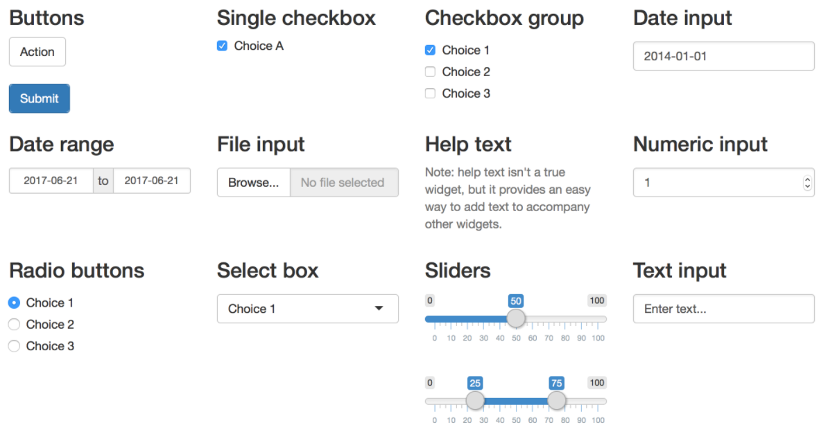
FIGURE 13.3: Examples of inputs.

To add an input to a Shiny app, we need to place an input function *Input() in the ui. Some examples of *Input() functions are

textInput() which creates a field to enter text,
dateRangeInput() which creates a pair of calendars for selecting a date range, and
fileInput() which creates a control to upload a file.

An *Input() function has a parameter called inputId with the id of the input, a parameter called label with the text that appears in the app next to the input, and other parameters that vary from input to input depending on its purpose. For example, a numeric input where we can enter numbers can be created by writing numericInput(inputId = "n", label = "Enter a number", value = 25). This input has id n, label “Enter a number” and default value equal to 25. The value of a specific input can be accessed by writing input$ and the id of the input. For example, the value of the numeric input with id n can be accessed with input$n. We can build an output in the server() function using input$n. Each time the user enters a number in this input, the input$n value changes and the outputs that use it update.

13.4 Outputs

Shiny apps can include a variety of output elements including plots, tables, texts, images and HTML widgets (Figure 13.4). HTML widgets are objects for interactive web data visualizations created with JavaScript libraries. Examples of HTML widgets are interactive web maps created with the leaflet package and interactive tables created with the DT package. HTML widgets are embedded in Shiny by using the htmlwidgets package (Vaidyanathan et al. 2023). We can use the values of inputs to construct output elements, and this causes the outputs to update each time input values are modified.

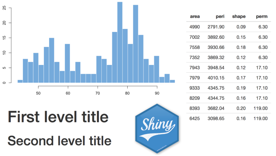
FIGURE 13.4: Examples of outputs.

Shiny provides several output functions *Output() that turn R objects into outputs in the user interface. For example,

textOutput() creates text,
tableOutput() creates a data frame, matrix or other table-like structure, and
imageOutput() creates an image.

The *Output() functions require an argument called outputId that denotes the id of the reactive element that is used when the output object is built in server(). A full list of input and output functions can be found in the Shiny reference guide.

13.5 Inputs, outputs and reactivity

As we have seen before, there are a variety of inputs and outputs that can be included in a Shiny app. Inputs are objects we can interact with by modifying their values such as texts, numbers or dates. Outputs are objects we want to show in the app and can be plots, tables or HTML widgets. Shiny apps use a functionality called reactivity to support interactivity. In this way, we can modify the values of the inputs, and automatically the outputs that use these inputs will change. The structure of a Shiny app that includes inputs and outputs, and supports reactivity is shown below.

ui <- fluidPage(
  *Input(inputId = myinput, label = mylabel, ...)
  *Output(outputId = myoutput, ...)
)

server <- function(input, output){
  output$myoutput <- render*({
    # code to build the output.
    # If it uses an input value (input$myinput),
    # the output will be rebuilt whenever
    # the input value changes
  })}

We can include inputs by writing an *Input() function in the ui. Outputs can be created by placing an output function *Output() in ui, and specifying the R code to build the output inside a render*() function in server().

The server() function has the arguments input and output. input is a list-like object that stores the current values of the inputs of the app. For example, input$myinput is the value of the input with id myinput defined in ui. output is a list-like object that stores the instructions for building the outputs of the app. Each element of output contains the output of a render*() function. A render*() function takes as an argument an R expression that builds the R object surrounded by curly braces {}. For example, output$hist <- renderPlot({ hist(rnorm(input$myinput)) }) creates a histogram with input$myinput values generated from a normal distribution. Examples of render*() functions are renderText() to create text, renderTable() to create data frames, matrices or other table like structures, and renderImage() to create images.

The output of a render*() function is saved in the output list. The object created with *Output() and render*() functions need to be of the same type. For example, to include a plot object, we use output$myoutput <- renderPlot({...}) in server() and plotOutput(outputId = "myoutput") in ui. Reactivity is created by linking the values of the inputs to the output elements. We can achieve this by including the value of an input (input$myinput) in the render*() expression. Thus, when we change the value of an input, Shiny will rebuild all the outputs that depend on that input using the updated input value.

13.6 Examples of Shiny apps

Here, we show the code to build the two Shiny apps of the previous examples, and explain how interactivity is created.

13.6.1 Example 1

The first Shiny app shows a numeric input and a histogram constructed with $n$ values that are randomly generated from a normal distribution (Figure 13.1). The number $n$ is given by the number that is introduced in the numeric input. Each time the user changes the number in the numeric input, the histogram is rebuilt. The content of the app.R file that generates this Shiny app is the following:

# load the shiny package
library(shiny)

# define the user interface object with the appearance of the app
ui <- fluidPage(
  numericInput(inputId = "n", label = "Sample size", value = 25),
  plotOutput(outputId = "hist")
)

# define the server function with instructions to build the
# objects displayed in the ui
server <- function(input, output) {
  output$hist <- renderPlot({
    hist(rnorm(input$n))
  })
}

# call shinyApp() which returns the Shiny app object
shinyApp(ui = ui, server = server)

The user interface ui contains a numericInput() function with id n that creates the numeric input. This input has label “Sample size” and default value equal to 25. The value that the user introduces in the numeric input can be accessed with input$n (that is, input$ followed by the input id n) and it denotes the number of values that will be generated from a normal distribution to construct the histogram. The ui also has a plotOutput() function with id hist and this function creates a place for the histogram that will be generated in the server() function. All elements of the user interface are placed inside the fluidPage() function and this creates a display that automatically adjusts the app to the dimensions of the browser window.

In the server() function, we write the code to build the outputs that are shown in the Shiny app. This function accepts inputs and computes outputs. The output output$hist (element hist in ui) is assigned a plot that is generated with the instruction hist(rnorm(input$n)). Thus, output$hist is a histogram of input$n values randomly generated with the rnorm() function. Here, input$n is the number introduced in the numeric input called n that is defined in the ui object. The code that generates the histogram is wrapped in a call to renderPlot() to indicate that the output is a plot.

Here we see that the code to build the plot uses input$n which is the value of the input with id n defined in the ui. This makes the plot reactive and each time we change the value of the input n, the histogram is rebuilt. Finally we call shinyApp() passing ui and server an this creates the Shiny app.

FIGURE 13.5: Snapshot of the first Shiny app.

13.6.2 Example 2

The second Shiny app shows a dropdown menu containing the names of world regions (North America, Europe, Asia, South America, Oceania, and Africa), and a bar plot with the number of telephones of the region selected in the dropdown in years 1951, 1956, 1957, 1958, 1959, 1960 and 1961 (Figure 13.2). In this app, each time the user selects a different region, the barplot is rebuilt. The data used in the app is the WorldPhones data of the datasets package. The app.R file to generate this Shiny app is the following:

# load the shiny package
library(shiny)

# load the datasets package wich contains the WorldPhones dataset
library(datasets)

# define the user interface object with the appearance of the app
ui <- fluidPage(
  selectInput(
    inputId = "region", label = "Region",
    choices = colnames(WorldPhones)
  ),
  plotOutput(outputId = "barplot")
)

# define the server function with instructions to build the
# objects displayed in the ui
server <- function(input, output) {
  output$barplot <- renderPlot({
    barplot(WorldPhones[, input$region],
      main = input$region,
      xlab = "Year",
      ylab = "Number of Telephones (in thousands)"
    )
  })
}

# call shinyApp() which returns the Shiny app object
shinyApp(ui = ui, server = server)

First, the packages shiny and datasets are attached. The ui object defines the appearance of the app. ui contains a selectInput() function with id region that creates the dropdown menu with the regions. The selectInput() function has label equal to “Region”, and choices equal to the list of possible regions in the data WorldPhones (choices = colnames(WorldPhones)). ui also contains a plotOutput() function with id barplot that creates a place for the barplot that will be generated in the server() function. ui is created by calling the fluidPage() function so the app automatically adjusts to the dimensions of the browser window.

The server() function contains the code to create the outputs shown in the ui. This function accepts inputs and computes outputs. The output output$barplot (element barplot in ui) is assigned a plot generated with the instruction barplot(WorldPhones[, input$region], ...). Here, input$region is the region selected in the input called region defined in the ui, and the barplot is computed with the values of the column input$region of WorldPhones. The title (main) of the barplot is the region given in input$region and the labels of the x and y axes are Year and Number of Telephones (in thousands), respectively. The code that generates the barplot is wrapped in a call to renderPlot() to indicate that the output is a plot. Finally, app.R includes the call shinyApp() with arguments ui and server and this creates the Shiny app.

FIGURE 13.6: Snapshot of the second Shiny app.

13.7 HTML content

The appearance of a Shiny app can be customized by using HTML content such as text and images. We can add HTML content with the shiny::tags object. tags is a list of functions that build specific HTML content. The names of the tag functions can be seen with names(tags). Some examples of tag functions, their HTML equivalents, and the output they create are the following:

h1(): <h1> first level header,
h2(): <h2> second level header,
strong(): <strong> bold text,
em(): <em> italicized text,
a(): <a> link to a webpage,
img(): <img> image,
br(): <br> line break,
hr(): <hr> horizontal line,
div: <div> division of text with a uniform style.

We can use any of these tag functions by subsetting the tags list. For example, to create a first level header we can write tags$h1("Header 1"), to create a link to a webpage we can write tags$a(href = "www.webpage.com", "Click here"), and to create a section in an HTML document we can use tags$div().

Some of the tag functions have equivalent helper functions that make accessing them easier. For example, the h1() function is a wrapper for tags$h1(), a() is equivalent to tags$a(), and div() is equivalent to tags$div(). However, most of the tag functions do not have equivalent helpers because they share a name with a common R function.

We can also include an HTML code different from the one that is provided by the tag functions. To do that, we need to pass a character string of raw HTML code to the HTML() function: tags$div(HTML("<strong> Raw HTML </strong>")). Additional information about tag functions can be found in Customize your UI with HTML and the Shiny HTML Tags Glossary.

13.8 Layouts

There are several options for creating the layout of the user interface of a Shiny app. Here, we explain the layout called sidebar. The specification of other layouts can be seen in the RStudio website. A user interface with a sidebar layout has a title, a sidebar panel for inputs on the left, and a main panel for outputs on the right. To create this layout, we need to add a title for the app with titlePanel(), and use a sidebarLayout() to produce a sidebar with input and output definitions. sidebarLayout() takes the arguments sidebarPanel() and mainPanel(). sidebarPanel() creates a a sidebar panel for inputs on the left, and mainPanel() creates a main panel for displaying outputs on the right. All these elements are placed within fluidPage() so the app automatically adjusts to the dimensions of the browser window as follows:

ui <- fluidPage(
  titlePanel("title panel"),
  sidebarLayout(
    sidebarPanel("sidebar panel"),
    mainPanel("main panel")
  )
)

We can rewrite the Shiny app of the first example using a sidebar layout. To do this, we need to modify the content of the ui. First, we add a title with titlePanel(). Then we include inputs and outputs inside sidebarLayout(). In sidebarPanel() we include the numericInput() function, and in mainPanel() we include the plotOutput() function. The Shiny app created with this layout has the numeric input on a sidebar on the left, and the histogram output on a large main area on the right (Figure 13.7).

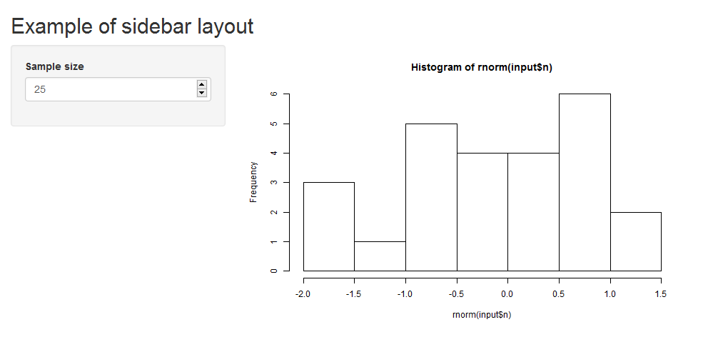
FIGURE 13.7: Snapshot of the first Shiny app with sidebar layout.

# load the shiny package
library(shiny)

# define the user interface object with the appearance of the app
ui <- fluidPage(
  titlePanel("Example of sidebar layout"),

  sidebarLayout(
    sidebarPanel(
      numericInput(
        inputId = "n", label = "Sample size",
        value = 25
      )
    ),

    mainPanel(
      plotOutput(outputId = "hist")
    )
  )
)

# define the server function with instructions to build the
# objects displayed in the ui
server <- function(input, output) {
  output$hist <- renderPlot({
    hist(rnorm(input$n))
  })
}

# call shinyApp() which returns the Shiny app object
shinyApp(ui = ui, server = server)

12 Building a dashboard to visualize spatial data with flexdashboard

14 Interactive dashboards with flexdashboard and Shiny