KAUST/ARAMCO Master’s in Data Science & Analytics Statistical Modeling of Data
Paula Moraga, Ph.D.
Prof. Statistics, KAUST
paula.moraga@kaust.edu.sa
Statistical Modeling of Data
Instructors
Professor Paula Moraga (Modules 1 - 4)
Professor Hernando Ombao (Modules 5 - 8)
Teaching Assistants
Ms. Mara Talento (Modules 1 - 4)
Ms. Farah Gomawi (Modules 5 - 8)
Course description
This course covers several topics essential to conducting data analysis. The goals are to train students
to conduct exploratory data analysis through visualization and summary statistics
to obtain confidence intervals and conduct tests of hypotheses
to build statistical general models, estimate parameters in these models, and model associations between outcome and explanatory variables
to conduct inference and forecasting in linear regression, logistic regression, categorical data analysis, and introductory time series and spatial analysis
Probability distributions and descriptive analysis
10:00 am - 10:45 am
Statistical inference and the Central Limit Theorem
10:45 am - 11:00 am
Coffee break
11:00 am - 12:00 pm
Confidence intervals
12:00 pm - 1:00 pm
Lunch break
1:00 pm - 2:30 pm
Hypothesis testing
2:30 pm - 2:45 pm
Coffee break
2:45 pm - 4:00 pm
Practical
Friday May 8: Linear regression and categorical variables
9:00 am - 10:00 am
Simple linear regression
10:00 am - 10:45 am
Multiple linear regression
10:45 am - 11:00 am
Coffee break
11:00 am - 12:00 pm
Break
12:00 pm - 1:00 pm
Lunch break
1:00 pm - 2:30 pm
Categorical variables
2:30 pm - 2:45 pm
Coffee break
2:45 pm - 4:00 pm
Practical
Saturday 9: Interactions, assumptions, and unusual observations
9:00 am - 10:45 am
Interactions
10:45 am - 11:00 am
Coffee break
11:00 am - 12:00 pm
Practical
12:00 pm - 1:00 pm
Lunch break
1:00 pm - 2:30 pm
Model assumptions and unusual observations
2:30 pm - 2:45 pm
Coffee break
2:45 pm - 4:00 pm
Practical
Sunday 10: Model selection, GLMs, and spatial analysis
9:00 am - 10:00 am
Model selection
10:00 am - 10:45 am
Introduction to Logistic and Poisson regression
10:45 am - 11:00 am
Coffee break
11:00 am - 12:00 pm
Practical
12:00 pm - 1:00 pm
Lunch break
1:00 pm - 2:30 pm
Spatial analysis
2:30 pm - 2:45 pm
Coffee break
2:45 pm - 3:30 pm
Practical
3:30 pm - 4:00 pm
Wrap-up
Evaluation
There will be two papers required for this course. Paper 1 will be on data analysis for the first half of the course, Paper 2 will be on the second half of the course. For each of the projects, students will analyze a dataset using the statistical techniques learned during the course. Students will need to submit a draft and a final written report, together with reproducible code.
Students will need to submit their work via Blackboard by the due date.
May 17 - deadline for Paper 1 draft (optional) May 31 - deadline for Paper 1 FINAL
June 18 - deadline for Paper 2 draft June 28 - deadline for Paper 2 FINAL
Grading
Paper 1: 10% draft + 40% final (If draft is not submitted, 50% final)
Paper 2: 10% draft + 40% final
Evaluation
Both papers 1 and 2 will include a title, abstract, introduction, data, methods, results and interpretation, a brief discussion section, and references. Make sure you accurately interpret your results, tables and figures in the context of the study. Tables and figures captions need to be self-contained.
For the reports, please use a maximum of 10 pages with 12 point font, one column, and 2cm margins, including tables and figures. Reports that exceed the specified number of pages will not be assessed. You will be judged on the quality and not on the quantity of material you submit.
You will need to submit via Blackboard a zip file containing the following:
written report
reproducible code and data. The code should load and analyze the data, work without errors, and include comments
Questions?
Probability distributions
Random variables
A random process is a random phenomenon or experiment that can have a range of outcomes. For example, tossing a coin, rolling a dice, or measuring the height of a randomly selected individual.
A random variable is a variable whose possible values are numbers associated to the outcomes of a random process.
Random variables are usually denoted with capital letters such as \(X\) or \(Y\).
Example
Random process: tossing a coin
Possible outcomes: heads and tails
Random variable: \(X\)
\(X =\) outcome when tossing a coin
\(X=1\) if heads and \(X = 0\) if tails
There are two types of random variables: discrete and continuous
A discrete random variable is one which may take only a finite or countable infinite set of values
\(X =\) outcome when tossing a coin (\(X=1\) if heads and \(X = 0\) if tails) \(X =\) number of members in a family randomly selected in a city (e.g., 2, 4, 6) \(X =\) number of patients admitted in a hospital in a given day \(X =\) number of defective light bulbs in a box of 20 \(X =\) year student randomly selected in the University was born (1998, 2000)
A continuous random variable is one which takes an infinite non-countable number of possible values
\(X\) = height student randomly selected in the department (1.65 m, 1.789 m) \(X\) = time required to run 1 Km (e.g., 4.56 min, 5.123 min) \(X\) = amount of sugar in an orange (e.g., 9.21 g, 12.2 g)
Probability distribution
A probability distribution of a random variable \(X\) is the specification of all the possible values of \(X\) and the probability associated with those values.
Probability mass function
If \(X\) is discrete, the probability distribution is called probability mass function
Value of \(X\)
\(P(X = x_i)\)
\(x_1\)
\(p_1\)
\(x_2\)
\(p_2\)
…
\(x_n\)
\(p_n\)
The probability mass function must satisfy
\(0 < p_i < 1\) for all \(i\), and \(\sum_{i=1}^n p_i = p_1 + p_2 + \ldots + p_n = 1\)
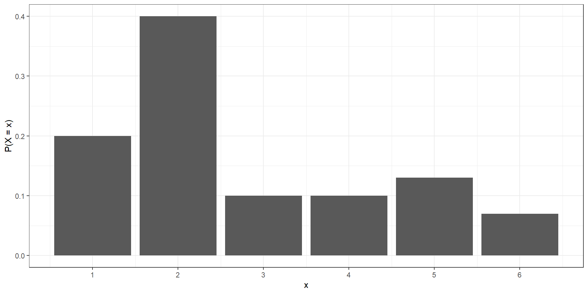
Example
\(X\) discrete random variable with the following probability mass function:
-
Outcome
1
2
3
4
5
6
Probability
0.20
0.40
0.10
0.10
0.13
0.07
Check the validity of the probability mass function
Calculate the probability that \(X\) is equal to 2 or 3
Calculate the probability that \(X\) is greater than 1
-
Outcome
1
2
3
4
5
6
Probability
0.20
0.40
0.10
0.10
0.13
0.07
Check the validity of the probability mass function
Probabilities between 0 and 1 and sum to 1
Calculate the probability that \(X\) is equal to 2 or 3
Calculate the probability that \(X\) is greater than 1
P(X > 1) = 1 - P(X = 1) = 1 - 0.2 = 0.8
Probability density function
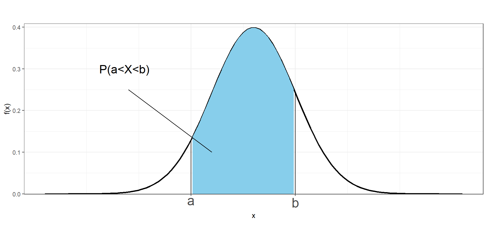
If \(X\) is continuous, the probability distribution is called probability density function. A continuous variable \(X\) takes an infinite number of possible values, and the probability of observing any single value is equal to 0, \(P(X = x) = 0\)
Therefore, instead of discussing the probability of \(X\) at a specific value \(x\), we deal with \(f(x)\), the probability density function of \(X\) at \(x\).
We cannot work with probabilities of \(X\) at specific values, but we can assign probabilities to intervals of values.
The probability of \(X\) being between \(a\) and \(b\) is given by the area under the probability density curve from \(a\) to \(b\).
\[P(a \leq X\leq b) = \int_a^b f(x)dx\]
The probability density function \(f(x)\) must satisfy the following:
The probability density function has no negative values (\(f(x) \geq 0\) for all \(x\))
Total area under the curve is equal to 1 (\(\int_{-\infty}^{+\infty} f(x)dx = 1\))
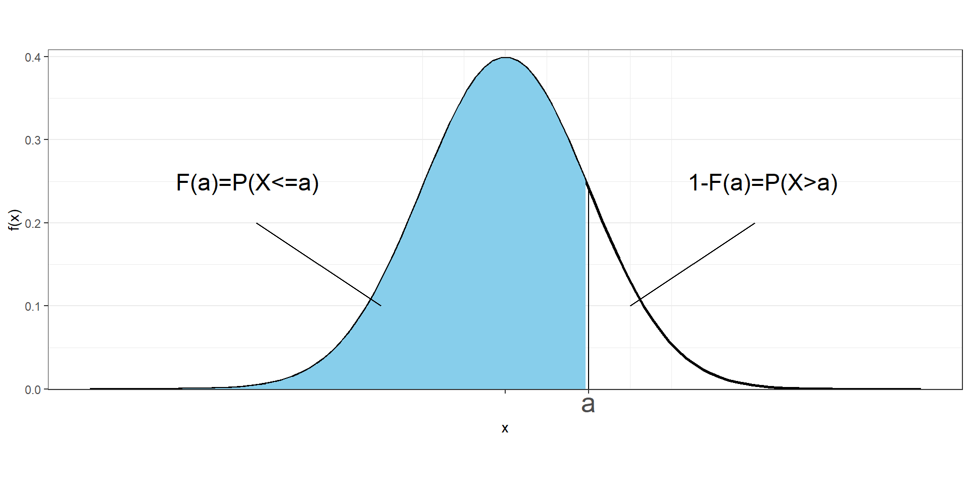
Cumulative distribution function
The cumulative distribution function (CDF) of a random variable \(X\) denotes the probability that \(X\) takes a value less than or equal to \(x\).
If \(X\) is discrete, the cumulative distribution function at a value \(x\) is calculated as the sum of the probabilities of the values that are less than or equal to \(x\):
\[F(x)=P(X\leq x) = \sum_{a\leq x}P(X=a)\]
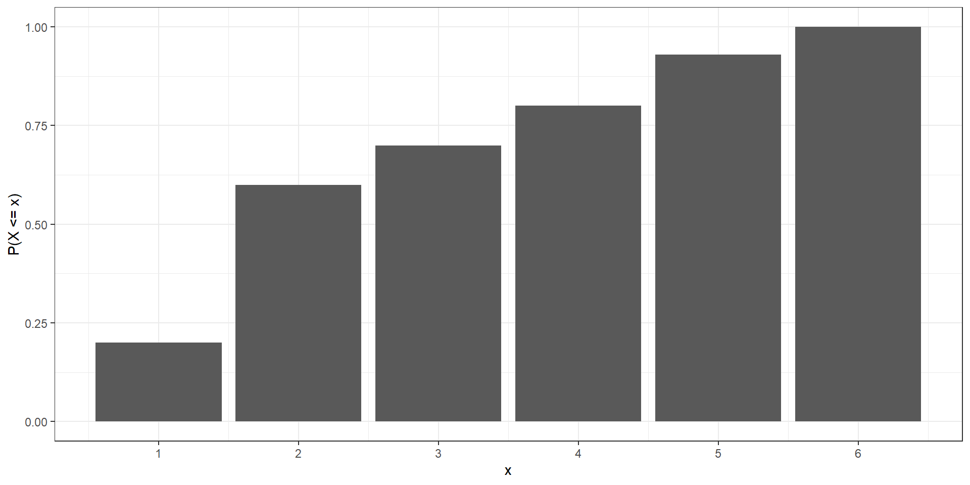
Example
Calculate the cumulative distribution function for the discrete random variable given by the following probability mass function:
-
Outcome
1
2
3
4
5
6
Probability
0.20
0.40
0.10
0.10
0.13
0.07
Example
Calculate the cumulative distribution function for the discrete random variable given by the following probability mass function:
-
Outcome
1
2
3
4
5
6
Probability
0.20
0.40
0.10
0.10
0.13
0.07
\(F(1) = P(X \leq 1) =\)
\(F(2) = P(X \leq 2) =\)
\(F(3) = P(X \leq 3) =\)
\(F(4) = P(X \leq 4) =\)
\(F(5) = P(X \leq 5) =\)
\(F(6) = P(X \leq 6) =\)
Example
Calculate the cumulative distribution function for the discrete random variable given by the following probability mass function:
If \(X\) is continuous, the cumulative distribution function at value \(x\) is calculated as the area under the probability density function to the left of \(x\)
\[F(x)=P(X\leq x) = \int_{-\infty}^x f(a)da\]
The probability that a continuous variable takes values between \(a\) and \(b\) is
\(P(a \leq X \leq b) = F(b) - F(a)\)
Bernoulli distribution
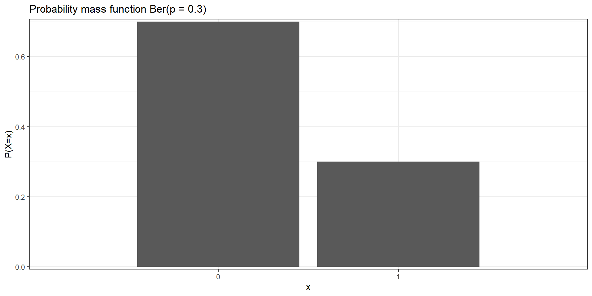
The Bernoulli distribution is used to describe experiments having exactly two outcomes (e.g., the toss of a coin will be head or tail, a person will test positive for a disease or not, or a political party will win an election or not).
\(X\) a random variable with Bernoulli distribution with probability of success \(p\)\[X \sim Ber(p)\]
Trial can result in two possible outcomes, success (\(X=1\))/ failure (\(X=0\))
Probability mass function: \(P(X = x) = p^x (1-p)^{1-x},\ x \in \{0, 1\}\) \(P(X=0) = p^0 (1-p)^{1-0}=1-p\) \(P(X=1) = p^1 (1-p)^{0}=p\)
Mean \(E[X]= \sum_{i} x_i P(X=x_i) = 0 (1-p)+ 1 p=p\)
Probability mass function: \(P(X = x) = p^x (1-p)^{1-x},\ x \in \{0, 1\}\)
\(P(X=0) = p^0 (1-p)^{1-0}=1-p = 1 - 0.3 = 0.7\)
\(P(X=1) = p^1 (1-p)^{0}=p = 0.3\)
Binomial distribution
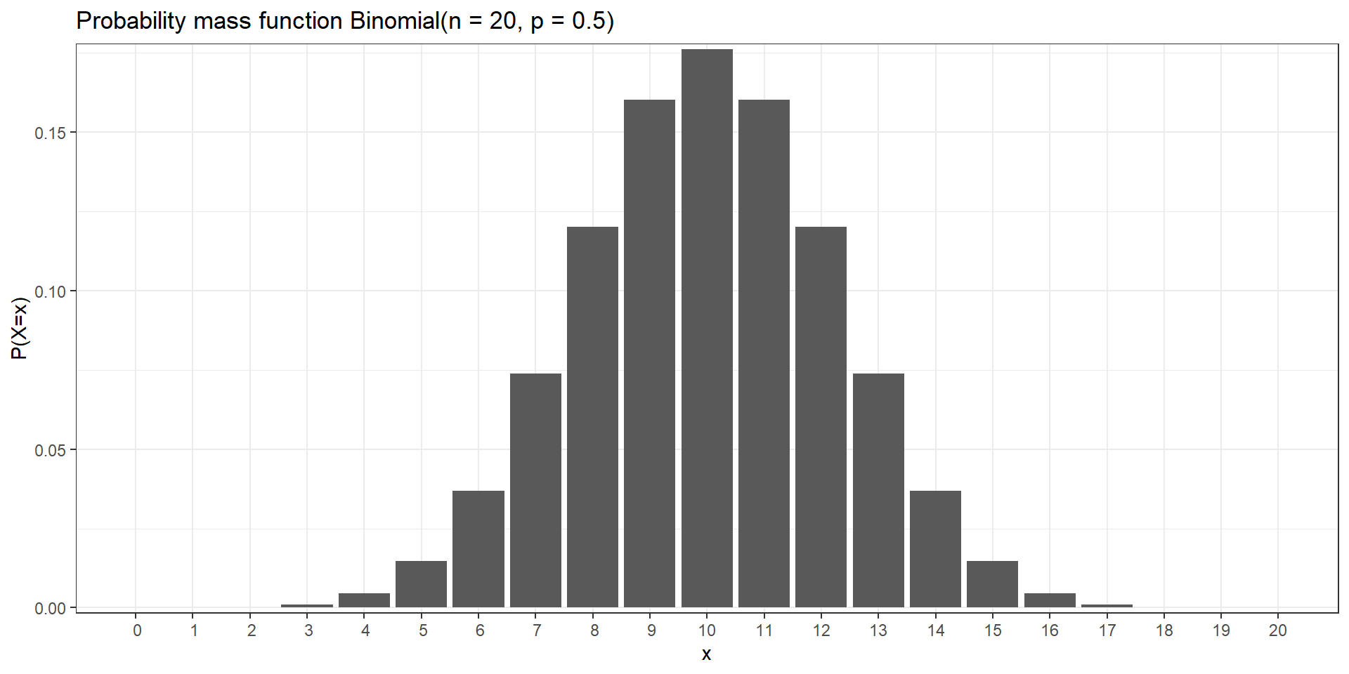
The binomial distribution is used to describe the number of successes in a fixed number of independent Bernoulli trials (e.g., number of heads when tossing a coin 20 times, number of defective pieces in a batch of 100 pieces)
\(X\) random variable with Binomial distribution with number of trials \(n\) and probability of success \(p\)
\[X \sim Binomial(n,p)\]
\(x=0,1,2,\ldots,n\) number of successes. \(n\) number of trials fixed
Probability of success \(p\) is the same from one trial to another
Each trial is independent (none of the trials have an effect on the probability of the next trial)
Probability mass function: \(P(X=x) = \binom{n}{x} p^x (1-p)^{n-x}\)
Mean is \(n p\). Variance is \(n p (1-p)\)
Example
Probability mass function: \(P(X=x) = \binom{n}{x} p^x (1-p)^{n-x}\)
 x            y
 0 9.536743e-07
 1 1.907349e-05
 2 1.811981e-04
 3 1.087189e-03
 4 4.620552e-03
 x          y
 5 0.01478577
 6 0.03696442
 7 0.07392883
 8 0.12013435
 9 0.16017914
  x          y
 10 0.17619705
 11 0.16017914
 12 0.12013435
 13 0.07392883
 14 0.03696442
  x            y
 15 1.478577e-02
 16 4.620552e-03
 17 1.087189e-03
 18 1.811981e-04
 19 1.907349e-05
 20 9.536743e-07
R syntax
Purpose
Function
Example
Generate n random values from a Binomial distribution
rbinom(n, size, prob)
rbinom(1000, 12, 0.25) generates 1000 values from a Binomial distribution with number of trials 12 and probability of success 0.25
Probability Mass Function
dbinom(x, size, prob)
dbinom(2, 12, 0.25) probability of obtaining 2 successes when the number of trials is 12 and the probability of success is 0.25
Cumulative Distribution Function (CDF)
pbinom(q, size, prob)
pbinom(2, 12, 0.25) probability of observing 2 or fewer successes when the number of trials is 12 and the probability of success is 0.25
Quantile Function (inverse of pbinom())
qbinom(p, size, prob)
qbinom(0.98, 12, 0.25) value at which the CDF of the Binomial distribution with 12 trials and probability of success 0.25 is equal to 0.98
Example
Let us consider a biased coin that comes up heads with probability 0.7 when tossed. Let \(X\) be the random variable denoting the number of heads obtained when the coin is tossed
What is the probability of obtaining 4 heads in 10 tosses?
Calculate \(P(X \leq 4)\)
Generate 3 random values from \(X \sim Bin(n = 10, p = 0.7)\)
\(X \sim Bin(n = 10, p = 0.7)\)
What is the probability of obtaining 4 heads in 10 tosses? \(P(X = 4)\)
Alternatively, using the cumulative distribution function
pbinom(4, size =10, prob =0.7)
[1] 0.04734899
Generate 3 random values from \(X \sim Bin(n = 10, p = 0.7)\)
rbinom(3, size =10, prob =0.7)
[1] 7 6 7
Normal distribution
The Normal distribution is used to model many procesess in nature and industry (e.g., heights, IQ scores, package delivery time, stock volatility)
\(X\) random variable with a normal distribution with mean \(\mu\) and variance \(\sigma^2\)
\[X \sim N(\mu, \sigma^2)\]
\(x \in \mathbb{R}\)
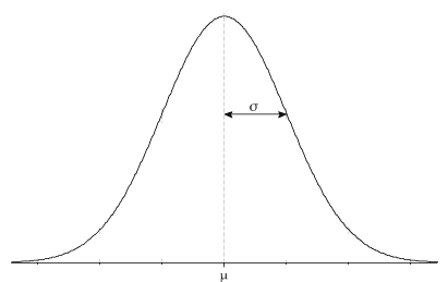
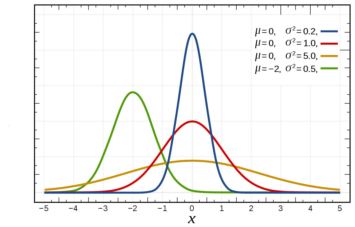
Probability density function: \(\displaystyle{f(x)=\frac{1}{\sigma \sqrt{2\pi}} exp^{-(x-\mu)^2/2 \sigma^2}}\)
Bell-shaped density function. Single peak at the mean (most data values occur around the mean). Symmetrical, centered at the mean
\(\mu \in \mathbb{R}\) represents the mean and the median of the normal distribution. The normal distribution is symmetric about the mean. Most values are around the mean, and half of the values are above the mean and half of the values below the mean. Changing the mean shifts the bell curve to the left or right.
\(\sigma>0\) standard deviation (\(\sigma^2>0\) variance). The standard deviation denotes how spread the data are. Changing the standard deviation stretches or constricts the curve.
Standard Normal distribution
The standard normal distribution is a normal distribution with mean 0 and variance 1.
The standard normal distribution is represented with the letter \(Z\). \[Z \sim N(\mu=0, \sigma^2=1)\]
If \(X \sim N(\mu, \sigma^2)\), then \(\displaystyle{Z = \frac{X-\mu}{\sigma} \sim N(0, 1)}\)
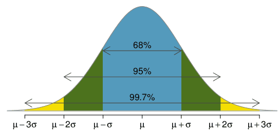
68-95-99.7 rule
The normal distribution is symmetric about the mean \(\mu\). Total area under probability density curve is 1. Probability below the mean is 0.5 and above 0.5.
Approximately 68% of the area lies between one standard deviation below the mean (\(\mu-\sigma\)) and one standard deviation above the mean (\(\mu+\sigma\)). Approximately 68% of data lies within 1 standard deviation from the mean.
Approximately 95% of data lies within 2 standard deviations from the mean.
Approximately 99.7% of data lies within 3 standard deviations from mean.
R syntax
Purpose
Function
Example
Generate n random values from a Normal distribution
rnorm(n, mean, sd)
rnorm(1000, 2, .25) generates 1000 values from a Normal distribution with mean 2 and standard deviation 0.25
Probability Density Function
dnorm(x, mean, sd)
dnorm(0, 0, 0.5) density at value 0 (height of the probability density function at value 0) of the Normal distribution with mean 0 and standard deviation 0.5.
Cumulative Distribution Function (CDF)
pnorm(q, mean, sd)
pnorm(1.96, 0, 1) area under the density function of the standard normal to the left of 1.96 (= 0.975)
Quantile Function (inverse of pnorm())
qnorm(p, mean, sd)
qnorm(0.975, 0, 1) value at which the CDF of the standard normal distribution is equal to 0.975 ( = 1.96)
Example
Consider a random variable \(X \sim N(\mu=100, \sigma=15)\). Calculate:
\(P(X < 125)\)
\(P(X \geq 110)\)
\(P(110 < X < 125)\)
Example
Consider a random variable \(X \sim N(\mu=100, \sigma=15)\). Calculate:
\(P(X < 125)\)
pnorm(125, mean =100, sd =15)
[1] 0.9522096
\(P(X \geq 110) = 1 - P(X < 110)\)
1-pnorm(110, mean =100, sd =15)
[1] 0.2524925
\(P(110 < X < 125) = P(X < 125) - P(X < 110)\)
pnorm(125, mean =100, sd =15) -pnorm(110, mean =100, sd =15)
[1] 0.2047022
Percentiles and quantiles
The \(k\)th percentile is the value \(x\) such that \(P(X < x) = k/100\).
The \(k\)th percentile of a set of values divides them so that \(k\)% of the values lie below and (100-\(k\))% of the values lie above.
Quantiles are the same as percentiles, but are indexed by sample fractions rather than by sample percentages (e.g., 10th percentile or 0.10 quantile).
Example
The mean Body mass index (BMI) for men aged 60 is 29 with a standard deviation of 6. BMI is expressed as kg/m^2. \(X \sim N(\mu=29, \sigma = 6)\)
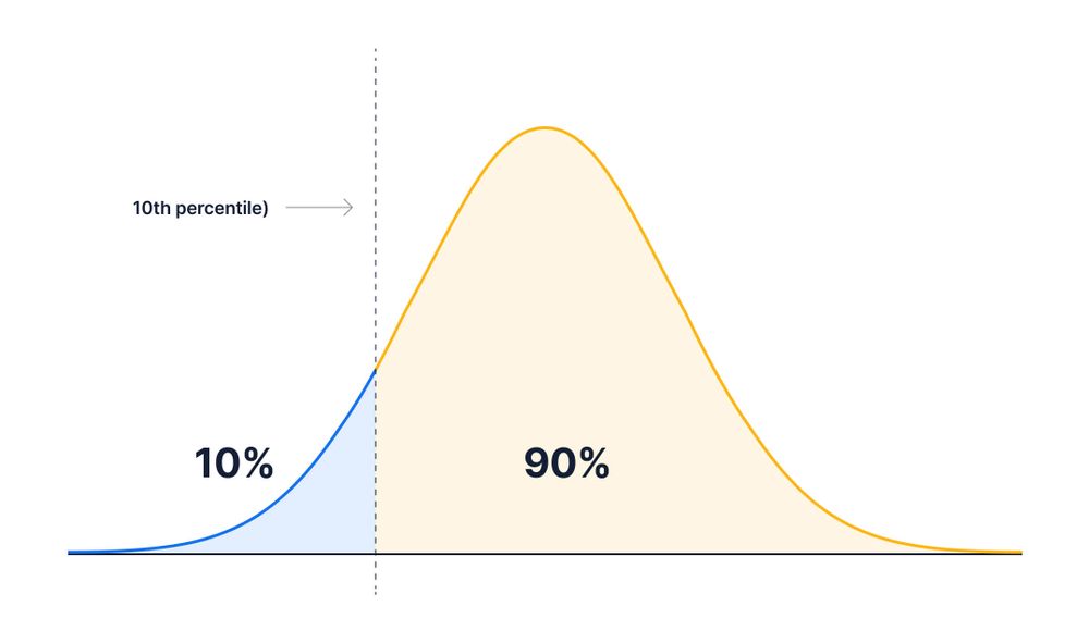
What is the 90th percentile (or quantile 0.90)?
The 90th percentile is the value \(x\) such that \(P(X < x) = 0.90\).
The 90th percentile is 36.69. This means 90% of the BMIs in men aged 60 are below 36.69. 10% of the BMIs in men aged 60 are above 36.69.
qnorm(0.90, mean =29, sd =6)
[1] 36.68931
Find percentile 25th (or quantile 0.25).
Value \(x\) such that \(P(X < x) = 0.25\).
qnorm(0.25, mean =29, sd =6)
[1] 24.95306
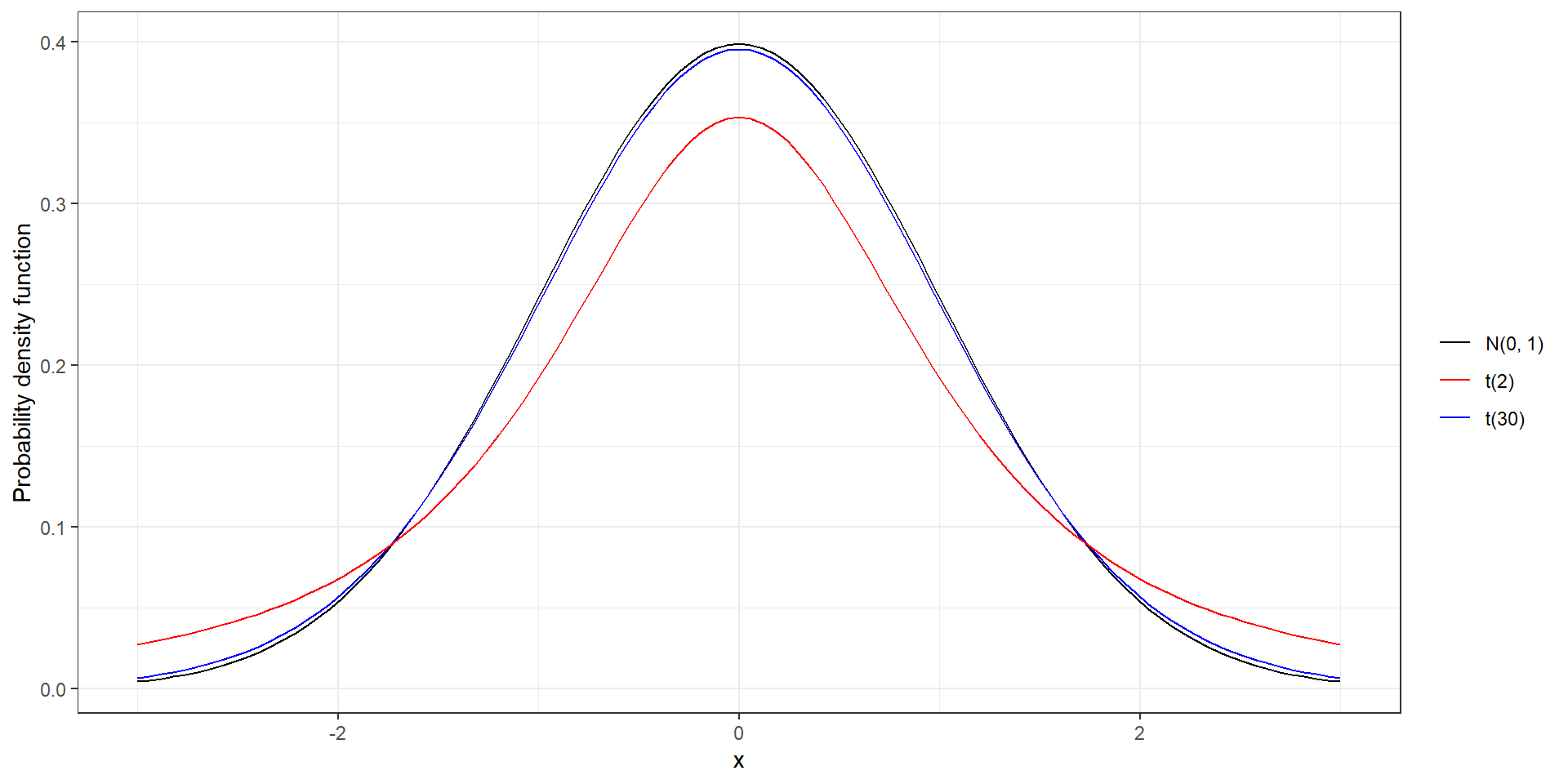
t distribution
Mean 0. Symmetric and bell-shaped like the normal distribution.
Heavier tails than normal distribution, observations more likely to fall beyond two standard deviations from the mean than under the normal
The t distribution has a parameter called degrees of freedom (df). The df describes the form of the t-distribution. When the number of degrees of freedom increases, the t-distribution approaches the standard normal, N(0, 1)
R syntax
Purpose
Function
Example
Generate n random values from a t distribution
rt(n, df)
rt(1000, 2) generates 1000 values from a t distribution with 2 degrees of freedom
Probability Density Function (PDF)
dt(x, df)
dt(1, 2) density at value 1 (height of the PDF at value 1) of the t distribution with 2 degrees of freedom
Cumulative Distribution Function (CDF)
pt(q, df)
pt(5, 2) area under the density function of the t(2) to the left of 5
Quantile Function (inverse of pt())
qt(p, df)
qt(0.97, 2) value at which the CDF of the t(2) distribution is equal to 0.97
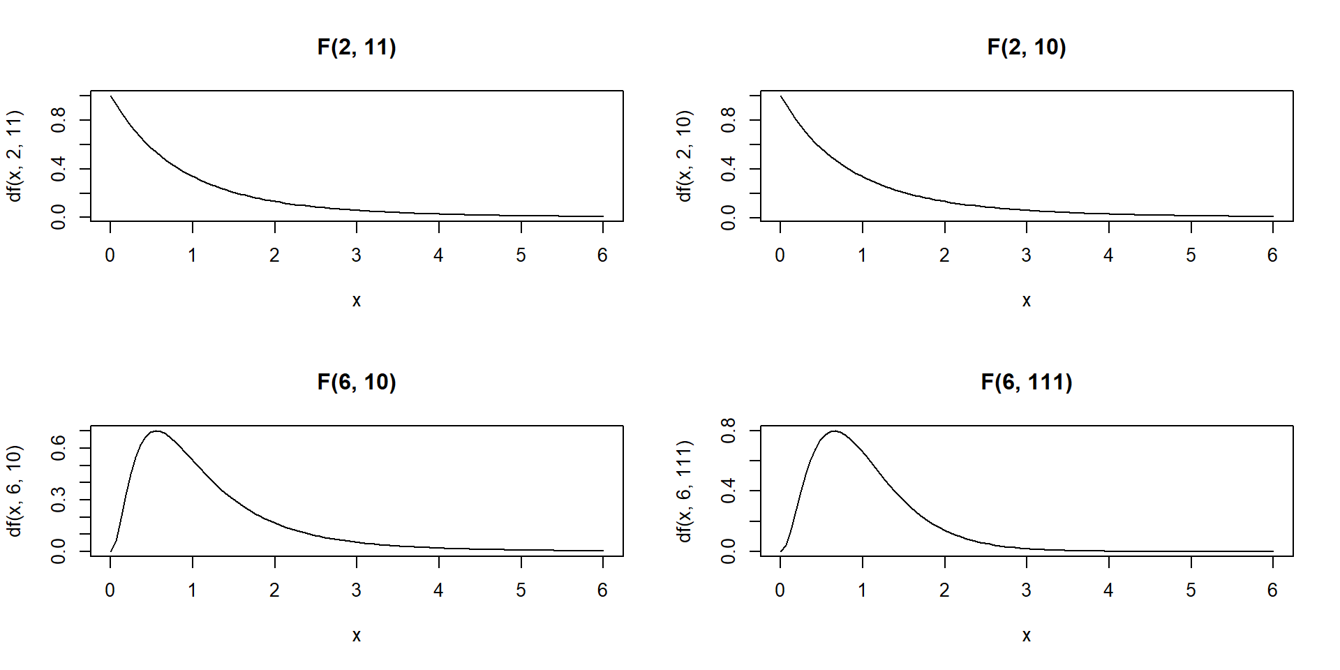
F distribution
The F distribution is usually defined as the ratio of variances of two populations normally distributed. The F distribution depends on two parameters: the degrees of freedom of the numerator and the degrees of freedom of the denominator.
The F-distribution is always \(\geq 0\) since it is the ratio of variances and variances are squares of deviations and hence are non-negative numbers.
Density is skewed to the right
Shape changes depending on the numerator and denominator degrees of freedom
As the degrees of freedom for the numerator and denominator get larger, the density approximates the normal
In ANOVA we always use the right-tailed area to calculate p-values
Density curves of four different F-distributions:
par(mfrow =c(2, 2)) # to draw figures in a 2 by 2 array on the devicex <-seq(0, 6, length.out =100)plot(x, df(x, 2, 11), main ="F(2, 11)", type ="l")plot(x, df(x, 2, 10), main ="F(2, 10)", type ="l")plot(x, df(x, 6, 10), main ="F(6, 10)", type ="l")plot(x, df(x, 6, 111), main ="F(6, 111)", type ="l")
R syntax
Purpose
Function
Example
Generate n random values from a F distribution
rf(n, df1, df2)
rf(1000, 2, 11) generates 1000 values from a F distribution with degrees of freedom 2 and 11
Probability Density Function (PDF)
df(x, df1, df2)
df(1, 2, 11) density at value 1 (height of the PDF at value 1) of the F distribution with degrees of freedom 2 and 11
Cumulative Distribution Function (CDF)
pf(q, df1, df2)
pf(5, 2, 11) area under the density function of the F(2,11) to the left of 5
Quantile Function (inverse of pf())
qf(p, df1, df2)
qf(0.97, 2, 11) value at which the CDF of the F(2,11) distribution is equal to 0.97
Find the 95th percentile (or quantile 0.95) of the F distribution with 2 and 11 degrees of freedom.
qf(0.95, df1 =2, df2 =11)
[1] 3.982298
Chi-squared distribution
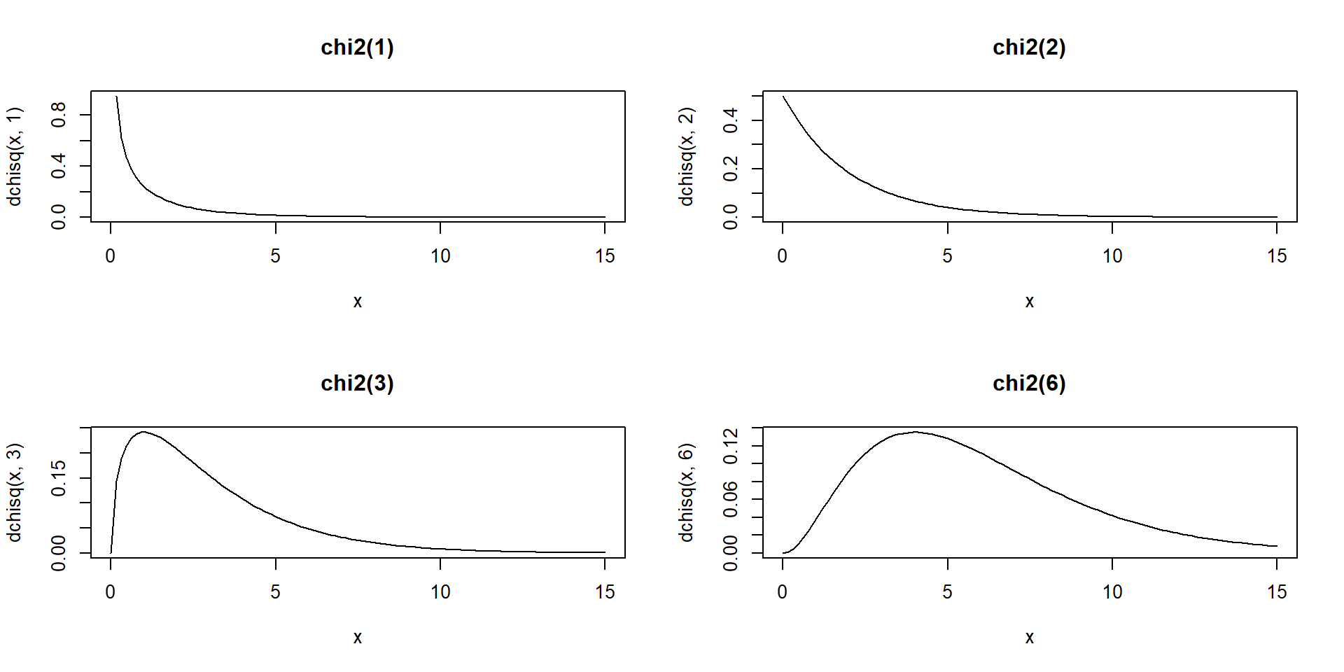
The chi-squared distribution with \(m \in N^*\) degrees of freedom is the distribution of a sum of squares of \(m\) independent standard normal random variables.
If \(X_1, X_2, \ldots, X_m\) are \(m\) independent random variables having the standard normal distribution, then \[V=X_1^2 + X_2^2+ \ldots + X_m^2 \sim \chi^2_{(m)}\] follows a chi-squared distribution with \(m\) degrees of freedom. Its mean is \(m\) and its variance is \(2m\).
Density curves of four different chi-squared distributions:
par(mfrow =c(2, 2)) # to draw figures in a 2 by 2 array on the devicex <-seq(0, 15, length.out =100)plot(x, dchisq(x, 1), main ="chi2(1)", type ="l")plot(x, dchisq(x, 2), main ="chi2(2)", type ="l")plot(x, dchisq(x, 3), main ="chi2(3)", type ="l")plot(x, dchisq(x, 6), main ="chi2(6)", type ="l")
R syntax
Purpose
Function
Example
Generate n random values from a chi-squared distribution
rchisq(n, df)
rchisq(1000, 2) generates 1000 values from a chi-squared distribution with degrees of freedom 2
Probability Density Function (PDF)
dchisq(x, df)
dchisq(1, 2) density at value 1 (height of the PDF at value 1) of the chi-squared distribution with degrees of freedom 2
Cumulative Distribution Function (CDF)
pchisq(q, df)
pchisq(5, 2) area under the density function of the chi-squared(2) to the left of 5
Quantile Function (inverse of pchisq())
qchisq(p, df)
qchisq(0.97, 2) value at which the CDF of the chi-squared(2) distribution is equal to 0.97
Find the 95th percentile (or quantile 0.95) of the chi-squared distribution with 6 degrees of freedom.
qchisq(0.95, df =6)
[1] 12.59159
Descriptive analysis
Descriptive statistics for continuous variables
Daily air quality measurements in New York, May to September 1973
There are three common measures of central tendency, all of which try to answer the basic question of which value is the most “typical.” These are the mean (average of all observations), median (middle observation), and mode (appears most often).
Sample Mean \[\bar x = \frac{\sum_{i=1}^n x_i}{n}\]
The central tendencies give a sense of the most typical values but do not provide with information on the variability of the values. Variability measures provide understanding of how the values are spread out.
min(d$Temp)
[1] 56
max(d$Temp)
[1] 97
Range corresponds to maximum value minus minimum value.
range(d$Temp)
[1] 56 97
max(d$Temp)-min(d$Temp)
[1] 41
Percentiles and quartiles answer questions like this: What is the temperature value such that a given percentage of temperatures is below it?
Specifically, for any percentage p, the pth percentile is the value such that a percentage p of all values are less than it. Similarly, the first, second, and third quartiles are the percentiles corresponding to p=25%, p=50%, and p=75%. These three values divide the data into four groups, each with (approximately) a quarter of all observations. Note that the second quartile is the median.
Quantiles are the same as percentiles, but are indexed by sample fractions rather than by sample percentages.
# default quantile() percentiles are 0% (minimum), 25%, 50%, 75%, and 100% (maximum)# provides same output as fivenum()quantile(d$Temp, na.rm =TRUE)
  0%  25%  50%  75% 100%
  56   72   79   85   97
# we can customize quantile() for specific percentilesquantile(d$Temp, probs =seq(from =0, to =1, by = .1), na.rm =TRUE)
Interquartile range (IQR) corresponds to the difference between the first and third quartiles.
# we can quickly compute the difference between the 1st and 3rd quantileIQR(d$Temp)
[1] 13
An alternative approach is to use the summary() function used to produce min, 1st quantile, median, mean, 3rd quantile, and max summary measures.
summary(d$Temp)
   Min. 1st Qu.  Median    Mean 3rd Qu.    Max.
  56.00   72.00   79.00   77.88   85.00   97.00
Variance. Although the range provides a measure of variability and percentiles/quartiles provide an understanding of divisions of the data, the most common measures to summarize variability are the variance and the standard deviation. They measure how spread out values are around their average.
     Ozone           Solar.R           Wind             Temp
 Min.   :  1.00   Min.   :  7.0   Min.   : 1.700   Min.   :56.00
 1st Qu.: 18.00   1st Qu.:115.8   1st Qu.: 7.400   1st Qu.:72.00
 Median : 31.50   Median :205.0   Median : 9.700   Median :79.00
 Mean   : 42.13   Mean   :185.9   Mean   : 9.958   Mean   :77.88
 3rd Qu.: 63.25   3rd Qu.:258.8   3rd Qu.:11.500   3rd Qu.:85.00
 Max.   :168.00   Max.   :334.0   Max.   :20.700   Max.   :97.00
 NA's   :37       NA's   :7
     Month            Day
 Min.   :5.000   Min.   : 1.0
 1st Qu.:6.000   1st Qu.: 8.0
 Median :7.000   Median :16.0
 Mean   :6.993   Mean   :15.8
 3rd Qu.:8.000   3rd Qu.:23.0
 Max.   :9.000   Max.   :31.0
Visualization
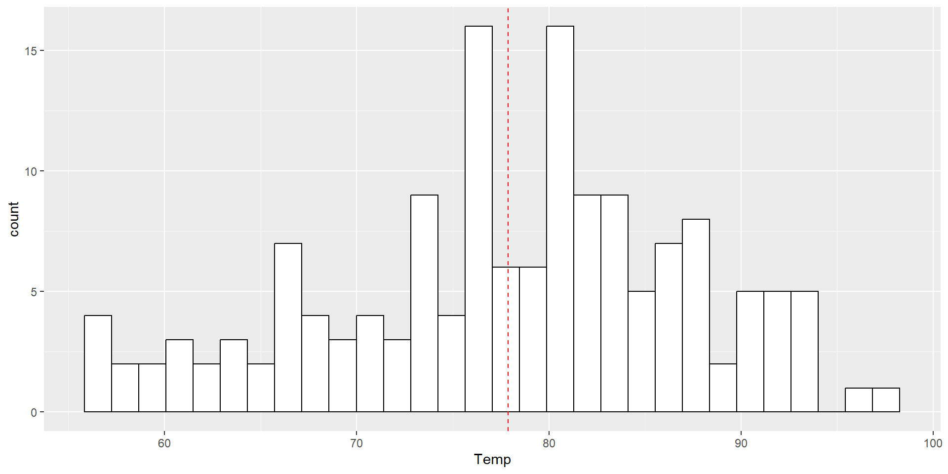
Histograms display a 1D distribution by dividing into bins and counting the number of observations in each bin. Whereas the previously discussed summary measures - mean, median, standard deviation, skewness - describes only one aspect of a numerical variable, a histogram provides the complete picture by illustrating the center of the distribution, the variability, skewness, and other aspects in one convenient chart.
hist(d$Temp)
library(ggplot2)ggplot(d, aes(Temp)) +geom_histogram(colour ="black", fill ="white") +geom_vline(aes(xintercept =mean(Temp)), color ="red", linetype ="dashed")
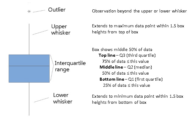
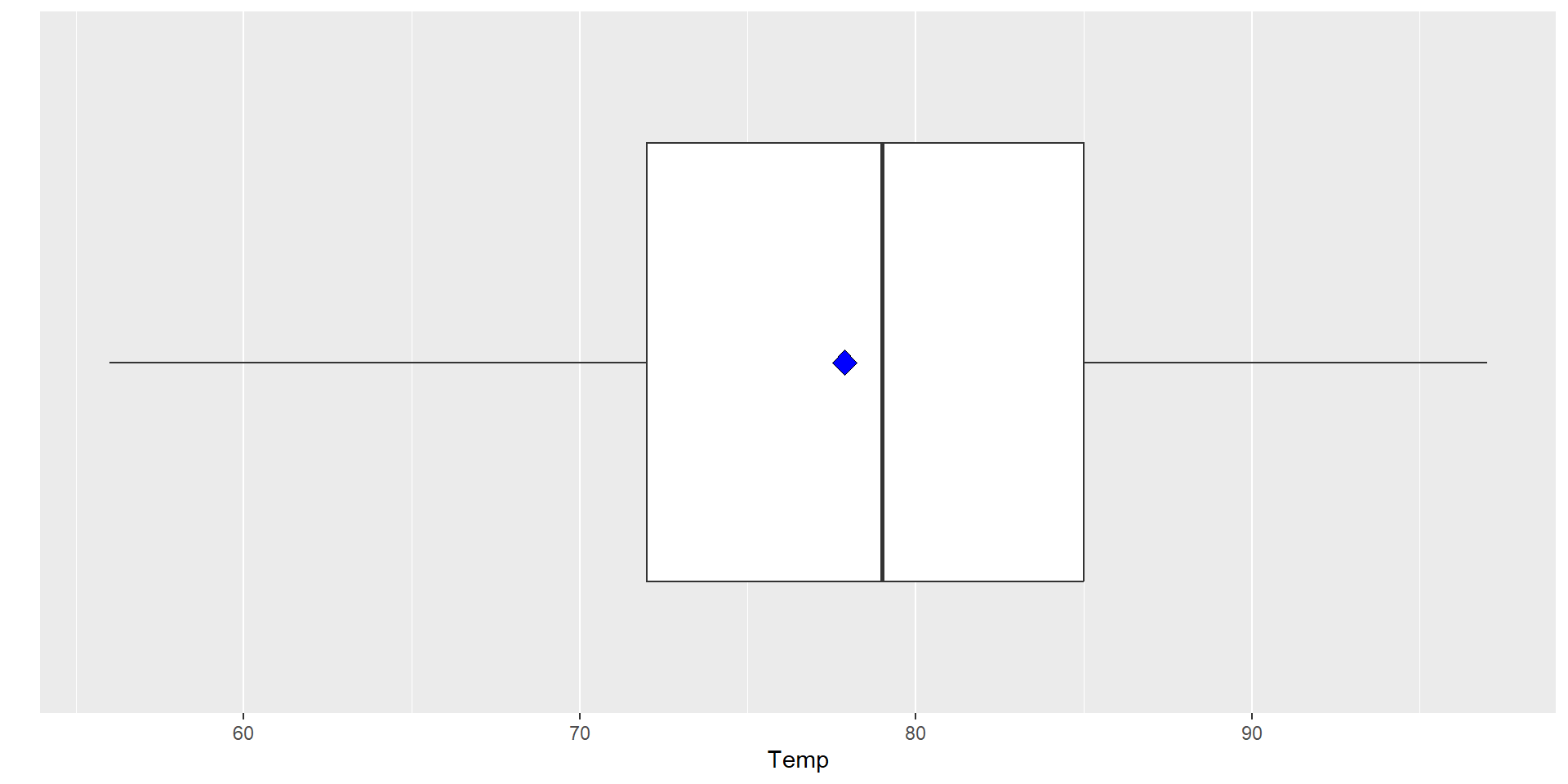
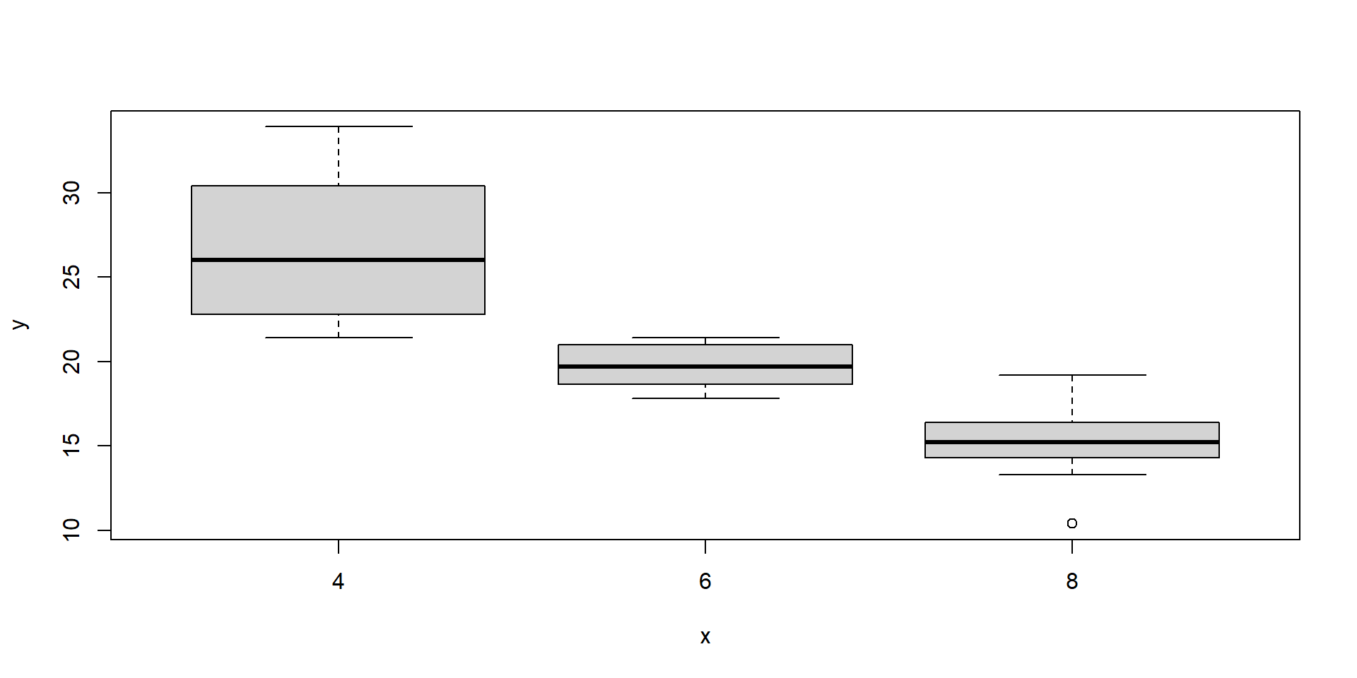
Boxplots
Boxplots are an alternative way to illustrate the distribution of a variable and is a concise way to illustrate the standard quantiles, shape, and outliers of data. The box itself extends from the first quartile to the third quartile. This means that it contains the middle half of the data. The line inside the box is positioned at the median. The lines (whiskers) coming out either side of the box extend to 1.5 interquartile ranges (IQRs) from the quartiles. These generally include most of the data outside the box. More distant values, called outliers, are denoted separately by individual points.
Fuel economy data from 1999 to 2008 for 38 popular models of cars
?ggplot2::mpg
library(ggplot2)d <- mpghead(d)
# A tibble: 6 × 11
  manufacturer model displ  year   cyl trans      drv     cty   hwy fl    class
  <chr>        <chr> <dbl> <int> <int> <chr>      <chr> <int> <int> <chr> <chr>
1 audi         a4      1.8  1999     4 auto(l5)   f        18    29 p     compa…
2 audi         a4      1.8  1999     4 manual(m5) f        21    29 p     compa…
3 audi         a4      2    2008     4 manual(m6) f        20    31 p     compa…
4 audi         a4      2    2008     4 auto(av)   f        21    30 p     compa…
5 audi         a4      2.8  1999     6 auto(l5)   f        16    26 p     compa…
6 audi         a4      2.8  1999     6 manual(m5) f        18    26 p     compa…
Frequencies and proportions for categorical variables
# counts for manufacturer categoriestable(d$manufacturer)
      audi  chevrolet      dodge       ford      honda    hyundai       jeep
        18         19         37         25          9         14          8
land rover    lincoln    mercury     nissan    pontiac     subaru     toyota
         4          3          4         13          5         14         34
volkswagen
        27
# percentages of manufacturer categoriestable2 <-table(d$manufacturer)prop.table(table2)
      audi  chevrolet      dodge       ford      honda    hyundai       jeep
0.07692308 0.08119658 0.15811966 0.10683761 0.03846154 0.05982906 0.03418803
land rover    lincoln    mercury     nissan    pontiac     subaru     toyota
0.01709402 0.01282051 0.01709402 0.05555556 0.02136752 0.05982906 0.14529915
volkswagen
0.11538462
Visualization
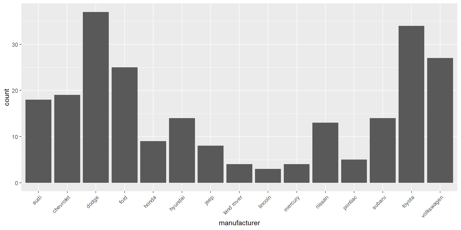
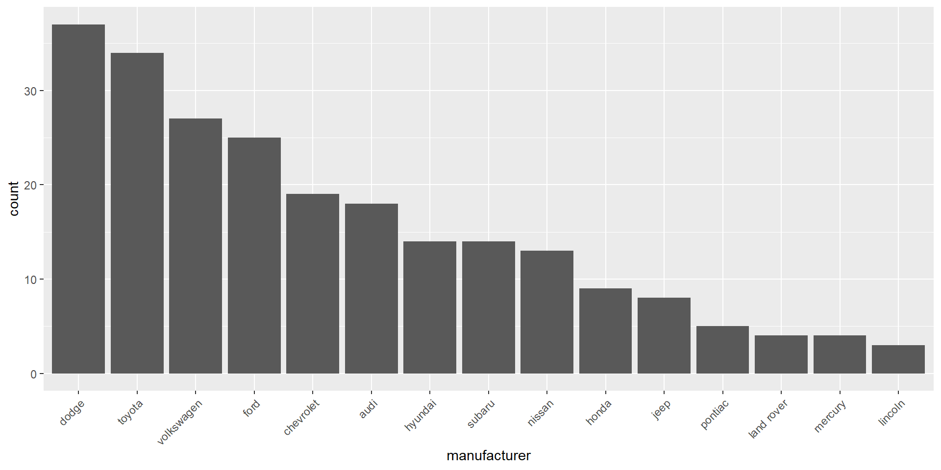
Bar charts are most often used to visualize categorical variables. Here we can assess the count of manufacturers:
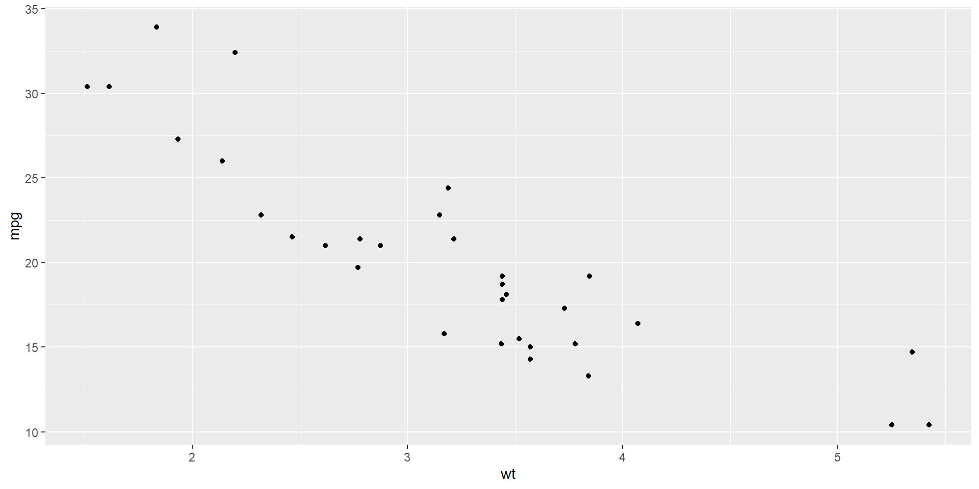
# if x is a factor it will produce a box plot# number of cylinders, milles per gallonplot(as.factor(mtcars$cyl), mtcars$mpg)
Statistical inference
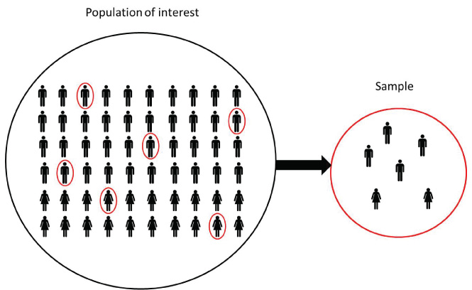
In statistical inference we are interested in learning some quantity representing some feature or parameter of a population. Population is large and we cannot examine all the values in the population directly. Therefore, to learn about the population parameter we take samples from the population and use the information in the samples to draw conclusions about the population.
Population parameters are fixed values. We rarely know the parameter values because it is often difficult to obtain measures from the entire population.
Sample statistics are quantities computed from the values in the sample. They are random variables because they vary from sample to sample.
We use sample statistics to draw conclusions about unknown population parameters.
Example
Suppose we are interested in knowing the mean height of the population living in Saudi Arabia. Population is large and we cannot measure the height of everybody directly. We can get an estimate of the mean height by taking sample of say, 5000 people, and measuring their heights. We can provide point estimates and interval estimates for population parameters.
Population mean is denoted by \(\mu\) and it is unknown
Sample size is \(n = 5000\)
Heights of people in the sample: \((x_1, x_2, \ldots, x_{5000})\)
Point estimate = estimate that specifies a single value of the population.
Sample statistic is the average heights of people in the sample: \(\bar x = \sum x_i/n\)
Interval estimate = estimate that specifies a range of plausible values for the population parameter. We are 95% confident the population mean \(\mu\) is within \((a, b)\)
Sampling distributions of sample statistics
A sample statistic is a random variable because it varies from sample to sample. The distribution of a sample statistic is called sampling distribution.
The sampling distribution of a sample statistic has mean approximately equal to the population mean and standard deviation called standard error (SE).
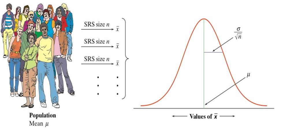
The Central Limit Theorem (CLT)
CLT states that for any given population distribution with mean \(\mu\) and standard deviation \(\sigma\), if we randomly take sufficiently large (\(n \geq 30\)) random samples from the population with replacement, the sampling distribution of the sample mean \(\bar X\) is normally distributed with mean \(\mu\) and standard error SE = \(\sigma/\sqrt{n}\).
\[\bar X \sim N\left(\mu, \frac{\sigma}{\sqrt{n}}\right)\]
Example
The mean height of a population is 160cm with standard deviation equal to 10. If we sample 50 people, what is the probability that the average height of the sample is greater than 170cm?
\(\bar X \sim N(\mu = 160, \sigma = 10/\sqrt{50})\)
The probability that the average height of the sample is greater than 170cm is \(P(\bar X > 170)\).
1-pnorm(170, mean =160, sd =10/sqrt(50))
[1] 7.687184e-13
Essentially 0, unlikely for the sample mean to exceed 170 given these parameters.
Simulation Central Limit Theorem
CLT states that for any given population distribution with mean \(\mu\) and standard deviation \(\sigma\), if we randomly take sufficiently large (\(n \geq 30\)) random samples from the population with replacement, the sampling distribution of the sample mean \(\bar X\) is normally distributed with mean \(\mu\) and standard error SE = \(\sigma/\sqrt{n}\).
\[\bar X \sim N\left(\mu, \frac{\sigma}{\sqrt{n}}\right)\]
Illustration of the Central Limit Theorem (CLT) by means of a simulation:
A \((c \times 100)\)% confidence interval for a population parameter based on sample observations is an interval \((A, B)\) such that we are \((c \times 100)\)% confident that the population parameter is within the interval.
When we use a different sample, we obtain a different confidence interval
If we take many samples from the population and calculate 95% CIs for each sample, then 95% of these CIs will contain the true population parameter.
A \((c \times 100)\)% confidence interval for a population parameter is \[\mbox{sample statistic $\pm$ critical value $\times$ SE}\]
Sample statistic used to estimate the population parameter.
Sample mean (\(\bar X\)) to estimate the population mean (\(\mu\))
Sample proportion (\(\hat P\)) to estimate the population proportion (\(p\))
Standard error SE is the standard deviation of the sampling distribution of the sample statistic
Critical value (\(z^*\), \(t^*(n-1)\)).
Measures the number of SE to be added and subtracted from the sample statistic to achieve the desired confidence level
Quantiles
\[X \sim N(\mu = 0, \sigma = 1)\]
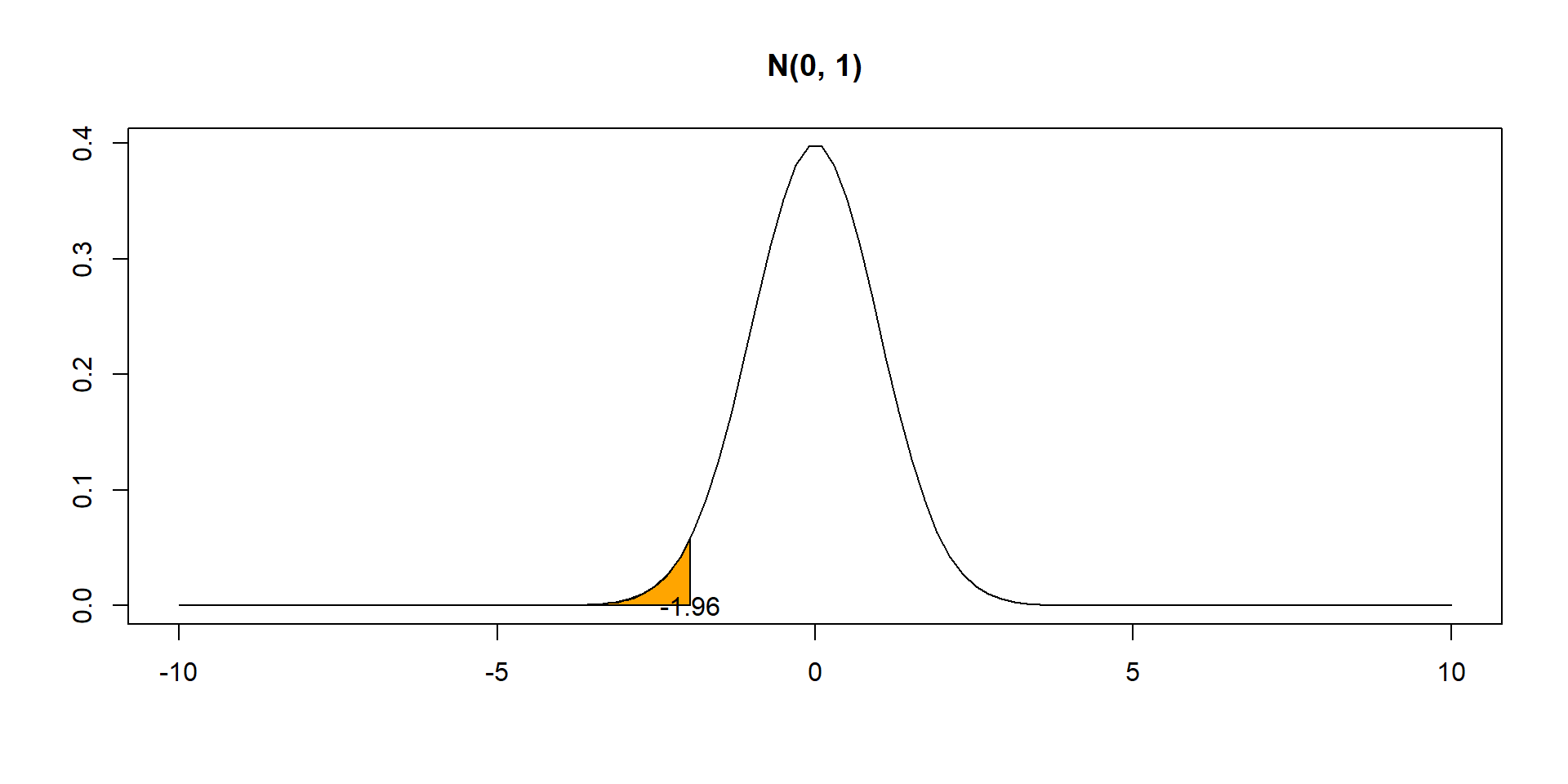
Find quantile 0.025. Value such that \(P(X < x) = 0.025\)
qnorm(0.025, mean =0, sd =1)
[1] -1.959964
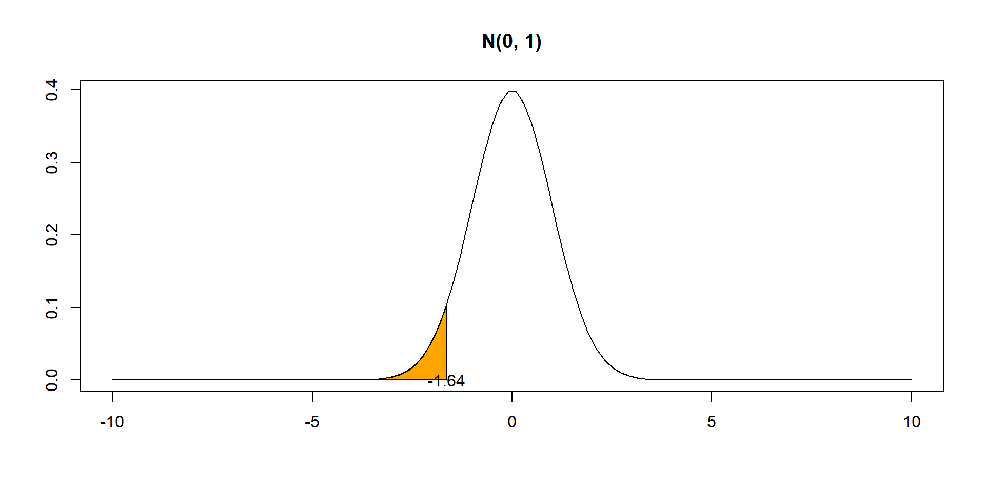
Find quantile 0.05. Value such that \(P(X < x) = 0.05\)
qnorm(0.05, mean =0, sd =1)
[1] -1.644854
Confidence interval for a proportion
Confidence interval for a proportion
\((1-\alpha) \times 100\)% confidence interval for the population proportion \(p\)\[\hat P \pm z^* \times SE = \hat P \pm z^* \times \sqrt{\hat P(1-\hat P)/n}\]
Assumptions:
Sample observations are independent (random sample)
In the sample, there are at least 10 successes and 10 failures
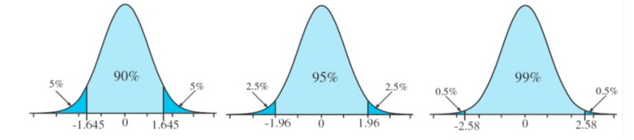
\(z^*\): value such that \(c=1-\alpha\) of the probability in the N(0,1) falls between \(-z^*\) and \(z^*\).
Value such that \(\alpha/2\) of the probability in the \(N(0,1)\) is below \(z^*\)
Example. Confidence interval for a proportion
In a random sample of 40 students, 24 said they bought a copy of the textbook. Estimate the proportion of all students who bought the book and give a 95% confidence interval.
Solution\[\hat p \pm z^* \times SE = \hat p \pm z^* \times \sqrt{\hat p(1-\hat p)/n}\] Assumptions:
Sample observations independent (random sample)
At least 10 successes (\(24 \geq 10\)) and 10 failures (\(40-24=16 \geq 10\))
Sample statistic: \(\hat p = 24/40 = 0.6\)
Critical value: \(z^* = -1.96\)
(\(\alpha/2\) of the probability in \(N(0,1)\) is below \(z^*\))
qnorm(0.025)
[1] -1.959964
\(\hat p \pm z^* \times SE = \hat p \pm z^* \times \sqrt{\hat p(1-\hat p)/n} = 0.6 \pm 1.96 \times \sqrt{ 0.6(1-0.6)/40} =\)\(= (0.448, 0.752)\)
An estimate of the proportion of students who bought the book is 60%.
We are 95% confident that the proportion of students is between 44.8% and 75.2%.
Confidence interval for a proportion
\((1-\alpha) \times 100\)% confidence interval for the population proportion \(p\)\[\hat P \pm z^* \times SE = \hat P \pm z^* \times \sqrt{\hat P(1-\hat P)/n}\]
Assumptions:
Sample observations are independent (random sample)
In the sample, there are at least 10 successes and 10 failures
\(z^*\): value such that \(c=1-\alpha\) of the probability in the N(0,1) falls between \(-z^*\) and \(z^*\).
Value such that \(\alpha/2\) of the probability in the \(N(0,1)\) is below \(z^*\)
\(\hat P\) is the proportion of successes in \(n\) trials. So \(\hat P\) is equal to \(Y/n\) where \(Y \sim Binomial(n, p)\).
\(Y\) can be expressed as the sum of \(n\) independent, identically distributed Bernoulli random variables, \[Y = \sum_{i=1}^n X_i\ \mbox{with } X_i \sim Ber(p),\ E[X_i]=p,\ Var[X_i]=p(1-p).\]
The Central Limit Theorem says that when we collect a sufficiently large sample of \(n\) independent observations, \(\bar X \sim N(\mu, \frac{\sigma}{\sqrt{n}})\). Thus, the sampling distribution of the sample proportion \(\hat P\)\[\hat P = \frac{\sum_{i=1}^n X_i}{n} \sim N\left(p, \mbox{SE = } \sqrt{\frac{p(1-p)}{n}}\right). \mbox{ We standardize } \hat P:\ \ \ Z = \frac{\hat P - p}{\sqrt{p(1-p)/n}} \sim N(0, 1)\]
\[P(-1.96 \leq \frac{\hat P - p}{\sqrt{\hat P(1-\hat P)/n}} \leq 1.96) = 0.95\] The probability is 95% that \(\hat P\) is within 1.96 standard errors of its mean
\[P(\hat P -1.96 \times {\sqrt{\hat P(1-\hat P)/n}} \leq p \leq \hat P + 1.96 \times {\sqrt{\hat P(1-\hat P)/n}}) = 0.95\]
A \((1-\alpha) \times 100\)% confidence interval for \(p\) is \[(\hat P -z^* \times {\sqrt{\hat P(1-\hat P)/n}},\ \hat P + z^* \times {\sqrt{\hat P(1-\hat P)/n}}). \mbox{ $z^*$ quantile $\alpha/2$}\]
\(z^*\) quantile \(\alpha/2\), value such \(\alpha/2\) of the probability in the N(0,1) distribution is below \(z^*\).
Example. Confidence interval for a proportion
A random sample of 826 people living in UK was surveyed to better understand their political preferences. 70% of the responses supported the political party A. Calculate a 95% confidence interval for the proportion of people that support the political party A.
Solution\[\hat p \pm z^* \times SE = \hat p \pm z^* \times \sqrt{\hat p(1-\hat p)/n}\]
Assumptions:
Observations are independent (they are from a random sample)
In the sample at least 10 support (\(n \hat p = 826 \times 0.70 = 578 \geq 10\) and at least 10 do not support (\(n(1- \hat p) = 826 \times (1-0.70) = 248 \geq 10\))
Sample statistic: \(\hat p = 24/40 = 0.70\)
Critical value: \(z^* = -1.96\)
(\(\alpha/2=0.05/2\) of the probability in \(N(0,1)\) is below \(z^*\))
qnorm(0.025)
[1] -1.959964
\(\hat p \pm z^* \times SE = \hat p \pm z^* \times \sqrt{\hat p(1-\hat p)/n} = 0.70 \pm 1.96 \times 0.016 = (0.669, 0.731)\)
We are 95% confident that the true proportion of people who support political party A is between 0.669 and 0.731.
Confidence interval for a mean
t distribution
Symmetric and bell-shaped like the normal distribution.
Mean 0, Heavier tails than the normal distribution. Observations are more likely to fall beyond two standard deviations from the mean than under the normal distribution.
The t-distribution has a parameter called degrees of freedom (df) that describes its form. When the df increases, the t-distribution approaches the standard normal N(0, 1)
Confidence interval for a mean
\((1-\alpha) \times 100\)% confidence interval for the population mean \(\mu\)\[\bar X \pm t_{n-1}^* \times SE = \bar X \pm t_{n-1}^* \times \frac{S}{\sqrt{n}}\]\(t^*_{n-1}\) value such that \(\alpha/2\) of the probability in \(t(n-1)\) is below \(t^*_{n-1}\)
Assumptions:
Sample observations are independent.
Sample observations from a normally distributed population or \(n \geq 30\)
When the population standard deviation is known:
\[\bar X \pm z^* \times SE = \bar X \pm z^* \times \frac{\sigma}{\sqrt{n}}\]
\(z^*\) value such that \(\alpha/2\) of the probability in the N(0,1) is below \(z^*\)
Example. Confidence interval for a mean
In a class survey, students are asked how many hours they sleep per night. In a sample of 52 students, the mean was 5.77 hours with a standard deviation of 1.572 hours. Construct a 95% confidence interval for the mean number of hours slept per night in the population from which this sample was drawn.
Solution
\(\sigma\) is unknown, we use \(s\) and a t distribution with \(n-1=52-1\) df \[\bar x \pm t^*_{51} \times SE = \bar x - t^*_{51} \times \frac{s}{\sqrt{n}}\]
Assumptions:
We assume data are independent
\(n \geq 30\)
Sample statistic: \(\bar x = 5.77\)
Critical value: \(t^*_{51}= -2.01\)
(\(\alpha/2=0.05/2\) of the probability in t(51) is below \(t^*_{51}\))
qt(0.025, 51)
[1] -2.007584
\(\bar x \pm t^*_{51} \times SE = \bar x \pm t^*_{51} \times \frac{s}{\sqrt{n}} = 5.77 \pm 2.01 \times \frac{1.572}{\sqrt{52}} = (5.33, 6.21)\).
We are 95% confident the population mean is between 5.33 and 6.21 hours.
Confidence interval for a mean
\((1-\alpha) \times 100\)% confidence interval for the population mean \(\mu\)\[\bar X \pm t_{n-1}^* \times SE = \bar X \pm t_{n-1}^* \times \frac{S}{\sqrt{n}}\]\(t^*_{n-1}\) value such that \(\alpha/2\) of the probability in \(t(n-1)\) is below \(t^*_{n-1}\)
Assumptions:
Sample observations are independent.
Sample observations from a normally distributed population or \(n \geq 30\)
When the population standard deviation is known:
\[\bar X \pm z^* \times SE = \bar X \pm z^* \times \frac{\sigma}{\sqrt{n}}\]
\(z^*\) value such that \(\alpha/2\) of the probability in the N(0,1) is below \(z^*\)
Confidence interval for a mean when \(\sigma\) is known
\[\mbox{Sampling distribution of } \bar X: \ \ \bar X \sim N\left(\mu, SE = \frac{\sigma}{\sqrt{n}}\right)\]
\[\mbox{We standardize } \bar X: \ \ Z = \frac{\bar X - \mu}{\sigma/\sqrt{n}} \sim N(0, 1)\]
\[P(-1.96 \leq \frac{\bar X - \mu}{\sigma/\sqrt{n}} \leq 1.96) = 0.95\]
The probability is about 95% that \(\bar X\) is within 1.96 standard errors of its mean
\[P(\bar X -1.96 \times \frac{\sigma}{\sqrt{n}} \leq \ \mu \leq \bar X + 1.96 \times \frac{\sigma}{\sqrt{n}}) = 0.95\] A \((1-\alpha) \times 100\)% confidence interval for \(\mu\) is \[(\bar X -z^* \times \frac{\sigma}{\sqrt{n}} , \bar X + z^* \times \frac{\sigma}{\sqrt{n}})\]
\(z^*\) quantile \(\alpha/2\), value such \(\alpha/2\) of the probability in the N(0,1) distribution is below \(z^*\)
Confidence interval for a mean when \(\sigma\) is not known
When population standard deviation is not known, we approximate it with the sample standard deviation and use a \(t\) distribution with \(n-1\) degrees of freedom.
\[T = \frac{\bar X - \mu}{S/\sqrt{n}} \sim t(n-1)\]
A \((1-\alpha) \times 100\)% confidence interval for \(\mu\) is \[(\bar X - t^*_{n-1} \frac{S}{\sqrt{n}},\
\bar X + t^*_{n-1} \frac{S}{\sqrt{n}})\]
\(t^*_{n-1}\) quantile \(\alpha/2\), value such \(\alpha/2\) of the probability in the \(t(n-1)\) distribution is below \(t^*_{n-1}\)
Example. Confidence interval for a mean
Elevated mercury concentrations are an important problem for both dolphins and other animals who occasionally eat them. Calculate a 95% CI for the average mercury content in dolphins using a sample of 19 dolphins in Japan. In the sample, \(n=19\), \(\bar x = 4.4\), \(s = 2.3\), minimum \(= 1.7\) and maximum \(= 9.2\)\(\mu\)g/wet gram (micrograms of mercury per wet gram of muscle).
Solution\(\sigma\) is unknown, we use \(s\) and a t distribution with \(n-1=19-1\) df \[\bar x \pm t^*_{18} \times SE = \bar x \pm t^*_{18} \times \frac{s}{\sqrt{n}}\]
Assumptions:
Independence seems reasonable because observations come from a random sample.
Normality seems reasonable because there are not clear outliers (all observations are within 2.5 standard deviations of the mean).
Sample statistic: \(\bar x = 4.4\)
Critical value: \(t^*_{18} = -2.10\)
(\(\alpha/2=0.05/2\) of the probability in the t(18) distribution is below \(t^*_{18}\))
qt(0.025, 18)
[1] -2.100922
\(\bar x \pm t^*_{18} \times SE = \bar x \pm t^*_{18} \times \frac{s}{\sqrt{n}} = 4.4 \pm 2.10 \times \frac{2.3}{\sqrt{19}} = (3.29, 5.51)\)
We are 95% confident the average mercury content in dolphins is between 3.29 and 5.51 \(\mu\)g/wet gram.
Interpretation of a confidence interval
The interpretation of a 95% CI constructed using a sample of size \(n\) is that if we take many samples of size \(n\) from the population, and calculate the 95% CIs for each sample, then we would expect 95% of these CI to contain the value of the population parameter
Hypothesis testing is a procedure to determine whether a claim about a population parameter is reasonable.
Currently accepted value of population mean age is 18.
Sample mean is 50, far from the currently accepted value 18.
So we reject the current belief that mean age is 18. The data provide evidence to say mean age is greater than 18.
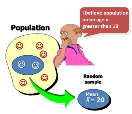
Currently accepted value of population mean age is 18.
Sample mean is 20, close to the currently accepted value 18.
So we fail to reject the current belief that mean age is 18. The data do not provide enough evidence to say mean age is greater than 18.
Hypothesis tests
Hypothesis testing is a procedure to determine whether a claim about a population parameter is reasonable.
Research question: Does a new drug reduce cholesterol?
The alternative or research hypothesis is the alternative to the currently accepted value for the population parameter
\(H_1\): The new drug reduces cholesterol
The null hypothesis represents “no difference” (currently accepted value of the population parameter)
\(H_0\): The new drug has no effect
To test a hypothesis, we select a sample from the population and use measurements from the sample and probability theory to determine how well the data and the null hypothesis agree.
We want to show the alternative hypothesis is reasonable (by showing there is evidence to reject the null hypothesis).
Example
Research question we are trying to answer
Does a new drug reduce cholesterol?
Alternative hypothesis (investigator’s belief) \(H_1\): The new drug reduces cholesterol
Null hypothesis (no difference, hypothesis to be rejected) \(H_0\): The new drug has no effect
Let \(\mu_1\) and \(\mu_2\) be the cholesterol levels obtained with and without the drug, respectively.
\(H_0: \mu_1 = \mu_2\) (Null hypothesis)
\(H_1: \mu_1 < \mu_2\) (Alternative hypothesis)
Null and alternative hypothesis
Null Hypothesis \(H_0\)
Alternative Hypothesis \(H_1\)
Assumed true until evidence indicates otherwise
We try to find evidence for the alternative hypothesis
“Nothing is going on”
Opposite of the null hypothesis
There is no relationship between variables being studied
There is relationship between variables being studied
An intervention does not make a difference/has no effect
An intervention makes a difference/has an effect
Hypothesis are written in terms of population parameters.
single mean (\(\mu\)), single proportion (\(p\)), difference between two independent means (\(\mu_1-\mu_2\)), diff between proportions (\(p_1-p_2\))
The null hypothesis \(H_0\) contains the equal sign (=)
Write the null and alternative hypothesis
Is the average monthly rent of a one-bedroom apartment in Madrid less than 800 Euros?
\(H_0\): \(\mu \geq 800\) \(H_1\): \(\mu < 800\)
Do the majority of all university students own a pet?
\(H_0: p \leq 0.5\) \(H_1: p > 0.5\)
In preschool, are the weights of boys and girls different?
\(H_0\): \(H_1\):
In preschool, are the weights of boys and girls different?
\(H_0: \mu_b = \mu_g\) \(H_1: \mu_b \neq \mu_g\)
Is the average intelligence quotient (IQ) score of all university students higher than 100?
\(H_0\): \(H_1\):
Is the proportion of men who smoke cigarettes different from the proportion of women who smoke cigarettes in England?
\(H_0\): \(H_1\):
Is the average intelligence quotient (IQ) score of all university students higher than 100?
\(H_0\): \(\mu \leq 100\) \(H_1\): \(\mu > 100\)
Is the proportion of men who smoke cigarettes different from the proportion of women who smoke cigarettes in England?
\(H_0: p_1 = p_2\) \(H_1: p_1 \neq p_2\)
Decisions in hypothesis testing
We make one of these two decisions:
Reject the null (if data provide evidence to disprove it)
Fail to reject the null (if data do not provide enough evidence to disprove it)
Failing to reject the null does not mean we accept the null. It is possible the data we have do not provide enough evidence against the null. But maybe we can collect additional data that provide evidence against the null.
A man goes to trial where he is being tried for a murder.
\(H_0\): Man is not guilty vs. \(H_1\): Man is guilty
It is possible the data we have do not provide enough evidence to reject the null and conclude the man is guilty. But we do not say he is innocent! We may collect additional data that provide evidence and then we can reject the null and say the man is guilty.
Errors in hypothesis testing
\(H_0\) is True
\(H_0\) is False
Reject null
Type I error
Correct
Fail to reject null
Correct
Type II error
Type I error: Reject the null hypothesis when it is true
Type II error: Fail to reject the null hypothesis when it is false
Example
\(H_0\): patient is not pregnant \(H_1\): patient is pregnant
Type I error: Reject the null hypothesis when it is true.
Patient is not pregnant but we conclude he is pregnant.
Type II error: Fail to reject the null hypothesis when it is false.
Patient is pregnant but we conclude she is not pregnant.
Example
A man goes to trial where he is being tried for a murder.
\(H_0\): Man is not guilty \(H_1\): Man is guilty
Type I error: Reject the null hypothesis when it is true.
Type II error: Fail to reject the null hypothesis when it is false.
Example
A man goes to trial where he is being tried for a murder.
\(H_0\): Man is not guilty \(H_1\): Man is guilty
Type I error: Reject the null hypothesis when it is true.
The man did not kill the person but was found guilty and was punished for a crime he did not really commit.
Type II error: Fail to reject the null hypothesis when it is false.
The man killed the person but was found not guilty and was not punished.
Significance level
Before testing the hypothesis, we select the significance level of the test \(\alpha\).
The significance level is the maximum probability of incorrectly rejecting the null when it is true we are willing to tolerate. Typical \(\alpha\) values are 0.05 and 0.01.
\(\alpha\) = P(Type I Error) = P(reject \(H_0\) | \(H_0\) is true)
If we choose \(\alpha = 0.05\), we have a maximum of 5% chance of incorrectly rejecting the null when it is true.
Steps in hypothesis testing
State the null and alternative hypotheses
Choose the significance level. Usually \(\alpha = 0.05\)
Calculate the test statistic using the sample observations \[\mbox{test statistic} = \frac{\mbox{sample statistic - null parameter}}{\mbox{standard error}}\]
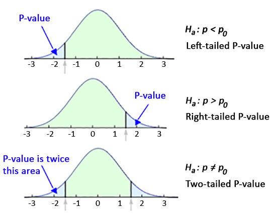
Find the p-value for the observed data
(p-value is the probability of obtaining a test statistic as extreme as or more extreme than the one observed in the direction of the alternative, assuming the null is true)
Make a decision and state a conclusion
If p-value < \(\alpha\), we reject the null
If p-value \(\geq \alpha\), we fail to reject the null
Example
A company manufacturing computer chips claims the defective rate is 5%. Let \(p\) denote the true defective probability. We use a sample of 1000 chips from the production to determine their claim is reasonable. The proportion of defectives in the sample is 8%.
1. State the null and alternative hypotheses
\(H_0: p = p_0\) (proportion of defective chips is 5%) \(H_1: p > p_0\) (proportion of defective chips is greater than 5%)
where \(p_0=0.05\)
2. Choose the significance level
We use a significance level \(\alpha = 0.05\)
So the maximum probability of incorrectly rejecting the null when it is true we are willing to tolerate is 5%.
The test statistic is a value calculated from a sample that summarizes the characteristics of the sample and is used to determine whether to reject or fail to reject the null hypothesis.
The test statistic differs from sample to sample. The sampling distribution of the test statistic under the null must be known so we can compare the results observed to the results expected from the null (e.g., test statistics with normal or t distributions).
Sampling distribution of the test statistic under the null hypothesis.
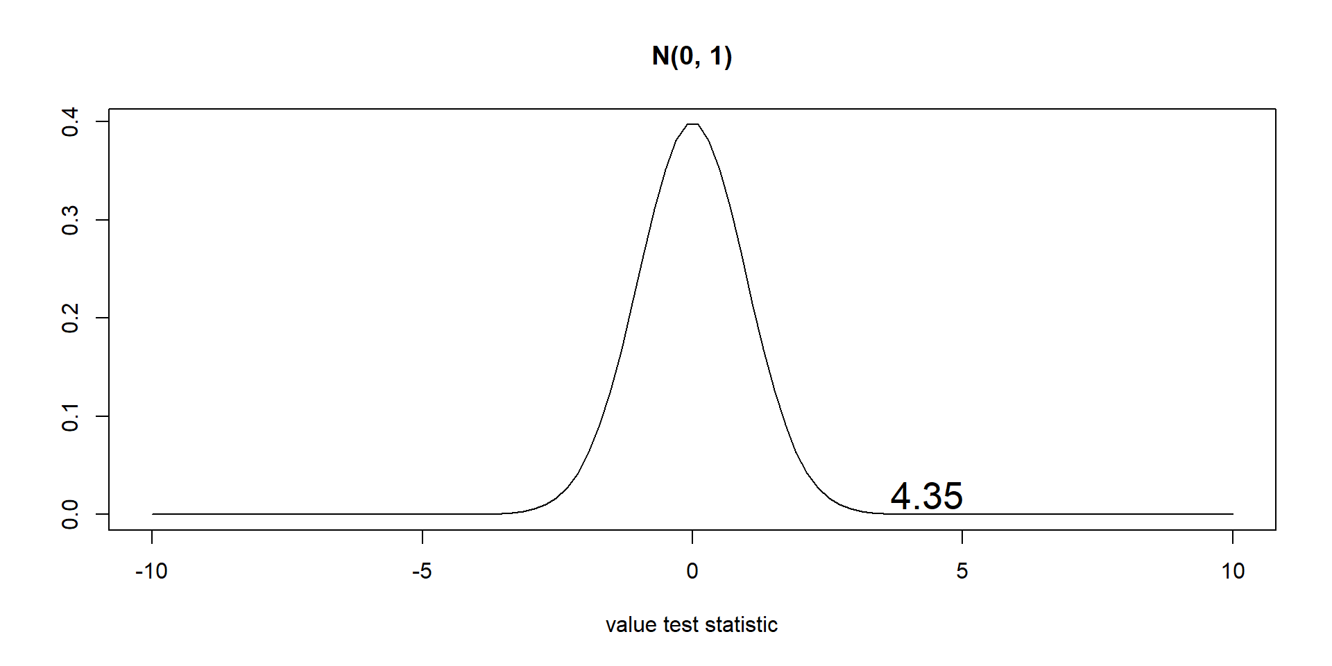
The value of the test statistic calculated with the sample observations is
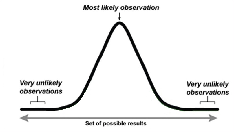
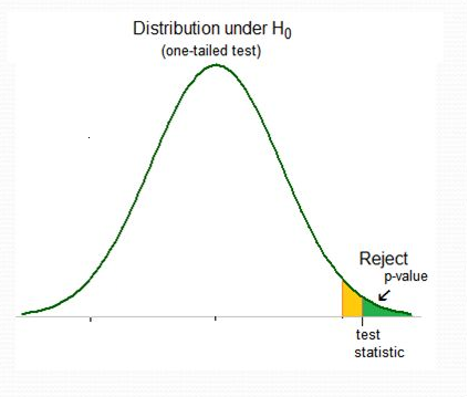
We reject the null if the observed value of the test statistic is so extreme that it is unlikely to occur if the null is true (unlikely to occur is given by the significance level \(\alpha\)). Otherwise we fail to reject the null.
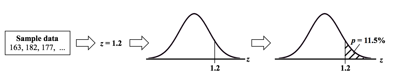
The p-value is the probability of obtaining a test statistic as extreme as or more extreme than the one observed in the direction of the alternative hypothesis, assuming the null hypothesis is true.
To calculate the p-value we compute the test statistic value using the sample data, and calculate the area under the test statistic distribution curve beyond the test statistic value.
5. Compare p-value and \(\alpha\) and make a decision
We compare the p-value to the significance level \(\alpha\) and decide whether to reject or fail to reject the null.
If p-value is small (p-value \(<\)\(\alpha\)) we had little chance of getting our data if the null hypothesis is true. So we reject the null. We conclude there is evidence against the null hypothesis.
If p-value is big (p-value \(\geq\)\(\alpha\)) there is reasonable chance of getting our data if the null hypothesis is true. So we fail to reject the null. We conclude there is not sufficient evidence against the null hypothesis.
1. State the null and alternative hypotheses
\(H_0: p = p_0\) (proportion of defective chips is 5%) \(H_1: p > p_0\) (proportion of defective chips is greater than 5%)
where \(p_0=0.05\)
2. Choose the significance level
We use a significance level \(\alpha = 0.05\)
So the maximum probability of incorrectly rejecting the null when it is true we are willing to tolerate is 5%.
3. Calculate the test statistic
Sample statistic is proportion of defective chips in the sample (\(\hat P\)).
Test statistic \[Z = \frac{\hat P - p_0}{\sqrt{\frac{p_0(1-p_0)}{n}}} \sim N(0,1)\]
The test statistic \(Z\) follows a N(0, 1) distribution under the null hypothesis (this holds if we have independent observations and the number of successes and failures are both greater than 10).