2 Statistical inference and the Central Limit Theorem
Learning objectives
- Population parameters and sample statistics
- Sampling distributions
- The Central Limit Theorem
2.1 Statistical inference
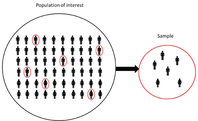
In statistical inference we are interested in learning some quantity representing some feature or parameter of a population. Population is large and we cannot examine all the values in the population directly. Therefore, to learn about the population parameter we take samples from the population and use the information in the samples to draw conclusions about the population.
Population parameters are fixed values. We rarely know the parameter values because it is often difficult to obtain measures from the entire population.
Sample statistics are quantities computed from the values in the sample. They are random variables because they vary from sample to sample.
We use sample statistics to draw conclusions about unknown population parameters.
Example
Suppose we are interested in knowing the mean height of the population living in England. Population is large and we cannot measure the height of everybody directly. We can get an estimate of the mean height by taking a sample of say, 5000 people, and measuring their heights.
We can provide point estimates and interval estimates for population parameters.
Population mean is denoted by \(\mu\) and it is unknown
Sample size is \(n = 5000\)
Heights of people in the sample: \((x_1, x_2, \ldots, x_{5000})\)
Point estimate = estimate that specifies a single value of the population.
Sample statistic is the average heights of people in the sample: \(\bar x = \sum x_i/n\)
Interval estimate = estimate that specifies a range of plausible values for the population parameter. We are 95% confident the population mean \(\mu\) is within \((a, b)\)
Example
A survey is carried out at a university to estimate the proportion of undergraduate students who drive to campus to attend classes. One thousand students are randomly selected and asked whether they drive or not to campus to attend classes. The population is all of the undergraduates at that university. The sample is the group of 1000 undergraduate students surveyed. The parameter is the true proportion of all undergraduate students at that university who drive to campus to attend classes. The statistic is the proportion of the 1000 sampled undergraduates who drive to campus to attend classes.
- Population proportion \(p\) unknown
- Sample size \(n = 1000\)
- Sample statistic is the sample proportion: \(\hat p = \frac{\mbox{number people drive}}{n}\)
Example
A study is conducted to estimate the true mean annual income of all adult residents of California. The study randomly selects 2000 adult residents of California. The population consists of all adult residents of California. The sample is the 2000 residents in the study. The parameter is the true mean annual income of all adult residents of California. The statistic is the mean income of the 2000 residents in this sample.
- Population mean \(\mu\) unknown
- Sample size \(n = 2000\)
- Sample statistic is the sample mean: \(\bar x = \sum x_i/n\)
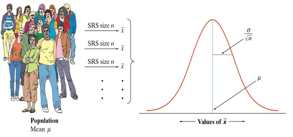
2.2 Sampling distributions of sample statistics
A sample statistic is a random variable because it varies from sample to sample. The distribution of a sample statistic is called sampling distribution.
The sampling distribution of a sample statistic has mean approximately equal to the population mean and standard deviation called standard error (SE).
Steps to construct the sampling distribution of a sample statistic (e.g., sample mean, sample proportion, etc.):
- Take a random sample of size \(n\) from the population
- For each sample, calculate the sample statistic (e.g., sample mean, sample proportion, etc.)
- Return the sample observations to the population and repeat the process many times
- If (theoretically) we choose every possible sample of size \(n\) from the population and calculate the sample statistic, we obtain the sampling distribution of the sample statistic
2.3 The Central Limit Theorem (CLT)
The Central Limit Theorem states that for any given population distribution with mean \(\mu\) and standard deviation \(\sigma\), if we randomly take sufficiently large (\(n \geq 30\)) random samples from the population with replacement, the sampling distribution of the sample mean \(\bar X\) is normally distributed with mean \(\mu\) and standard error SE = \(\sigma/\sqrt{n}\).
When we choose many random samples from a population, the sampling distribution of the sample mean \(\bar X\) is centered at the population mean \(\mu\) and is less spread out than the population distribution.
\[\bar X \sim N\left(\mu, \frac{\sigma}{\sqrt{n}}\right)\]
Example
Consider a sample of size \(n=40\) from a population with mean \(\mu = 30\) and standard deviation \(\sigma=10\). What are the mean and standard deviation of the sample mean?
Solution:
\(\mu_{\bar X} = \mu = 30\)
\(\sigma_{\bar X} = \sigma/\sqrt{n} = 10/\sqrt{40}\)
\(\bar X \sim N(\mu = 30, \sigma = 10/\sqrt{40})\)
Example
The mean height of a population is 160cm with standard deviation equal to 10. If we sample 50 people, what is the probability that the average height of the sample is greater than 170cm?
Solution:
\(\mu_{\bar X} = \mu = 160\)
\(\sigma_{\bar X} = \sigma/\sqrt{n} = 10/\sqrt{50}\)
\(\bar X \sim N(\mu = 160, \sigma = 10/\sqrt{50})\)
The probability that the average height of the sample is greater than 170cm is \(P(\bar X > 170)\).
2.3.1 Simulation Central Limit Theorem
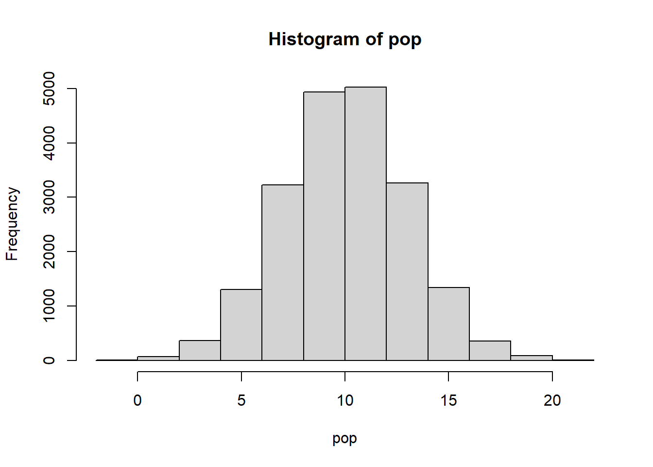
Consider a population with mean \(\mu = 10\) and standard deviation \(\sigma = 3\) (size N = 20000).
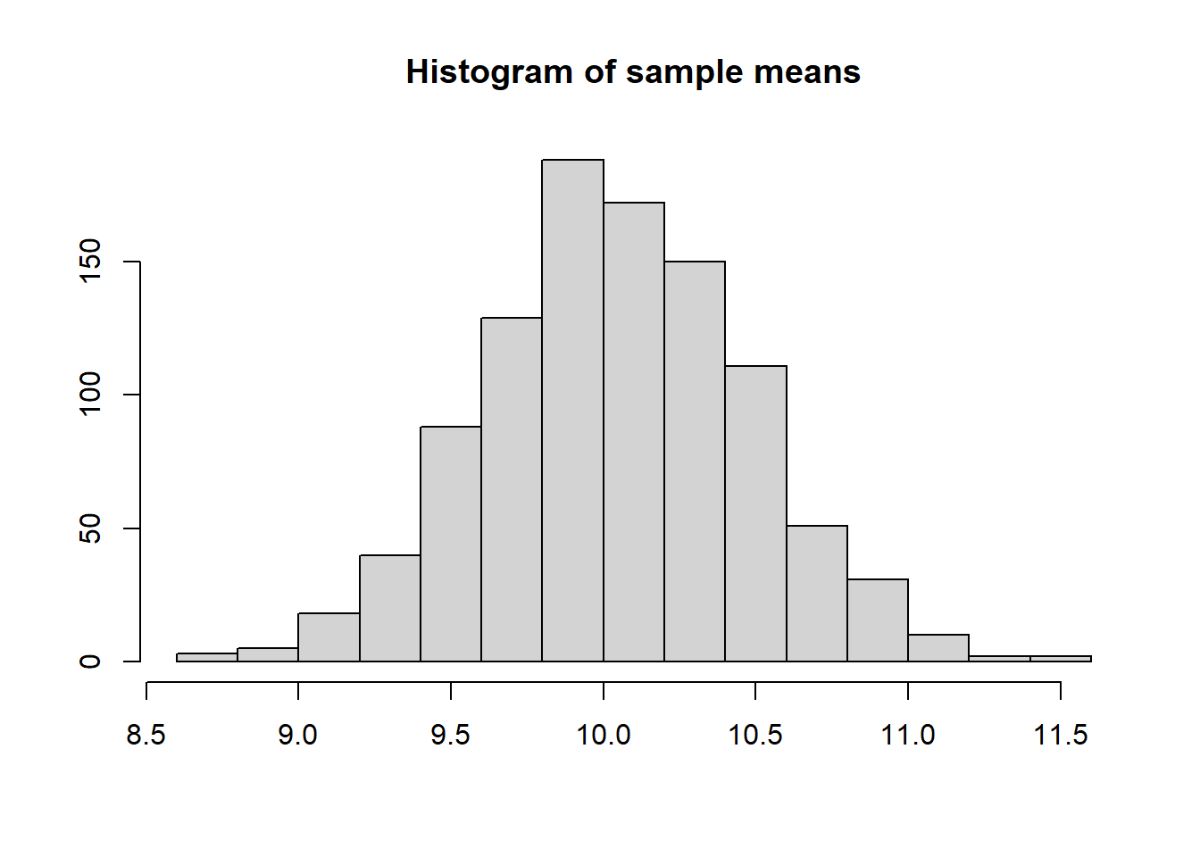
Choose a large number of samples of size \(n=50\) from the population
Sample 1
 [1]  7.975375 12.257470 10.377354  9.907790 11.937278  7.468786 11.762438
 [8]  8.206469  9.190119  8.944716  9.200704  9.527427  6.734539  8.512795
[15] 11.236278 10.535814  8.233852 10.080207  9.405853  8.554898  7.368190
[22] 13.406363  6.908683 12.533212 12.950893 10.695961  6.852835  6.570246
[29] 11.041544  7.120459 11.553031  8.761647  6.445764  8.352635  7.638423
[36] 12.769382 10.992989  5.946781 11.110433 11.355585  8.124870 15.255030
[43]  9.702626 12.666557 11.388436  7.739810 14.762229  8.790677 13.792156
[50] 14.047205
Sample 2
 [1]  8.196499  8.882126  6.400632  9.589160  9.969405 12.174885 11.199701
 [8] 11.732504 11.076944  6.765168 11.812206  8.296639  7.833411 10.775071
[15] 13.927455 16.505756 11.142394  7.281917  8.071225 10.596691  4.517464
[22]  9.549846 11.612885  8.918850  8.289792 17.985239 10.979836  2.165236
[29] 13.952113 11.696020 13.712214 11.708949 13.333695  9.387240 12.674901
[36]  4.398816  4.230698 11.706863  9.290259 13.214196  7.914871 11.533189
[43] 11.917677  3.955421  9.488963  6.281973 12.263498 11.908846  8.809323
[50]  7.584949
…
Sample 1000
 [1] 13.5556165  6.9131280 12.3085046 12.1246957  9.9142180 10.7900062
 [7]  7.0470766  6.6408230 10.2313240 13.8551990 11.5933873 12.6767345
[13] 11.2607703 12.6890528 14.6375235  0.6793787  7.9431965  9.4630750
[19] 11.9359139  6.8532437 11.2822946  5.9973758  9.1415962 12.6681362
[25] 12.5597843 13.2419490 12.7046971  9.7049784 13.1168152 14.5012611
[31] 12.2218530 11.5654120 10.0508732  8.6211252 12.2151162 11.2393961
[37]  1.6618359  7.3041759 11.5152791  8.9973111 13.2327804 11.4601462
[43]  9.8979077  9.3200936 12.6910851  7.7835314  7.5527052 13.2730664
[49] 14.9765053 12.4261288
Calculate sample means
\(\bar X\) sample 1
[1] 9.933896\(\bar X\) sample 2
[1] 9.944272…
\(\bar X\) sample 1000
[1] 10.52076- The mean of the sample means is equal to the mean of the population. \[\mu_{\bar X} = \mu\] (independent of sample size)
\(\mu_{\bar X}\)
[1] 9.972362\(\mu\)
[1] 9.974479- The standard deviation of sample means is equal to the standard deviation of the population divided by the square root of the sample size \[\sigma_{\bar X} =\frac{\sigma}{\sqrt{n}}\]
\(\sigma_{\bar X}\)
[1] 0.4102202\(\frac{\sigma}{\sqrt{n}}\)
[1] 0.4219211If the population is normal, then the sample means will have a normal distribution
If the population is not normal (can be skewed, discrete, etc) but the sample is sufficiently large (\(n \geq 30\)), then the sampling distribution of sample means approximates a normal distribution.
Sampling distribution of sample means
2.3.2 Simulation Central Limit Theorem
We illustrate the Central Limit Theorem (CLT) by means of a simulation. The CLT applies to any distribution. To illustrate the CLT we can consider any population, it does not necessarily need to be normal. For example, we consider the following population which consists of 100000 numbers drawn from two different normal distributions.
pop <- c(rnorm(20000, mean = 10, sd = 3),
         rnorm(80000, mean = 70, sd = 10))

hist(pop, main = "Population")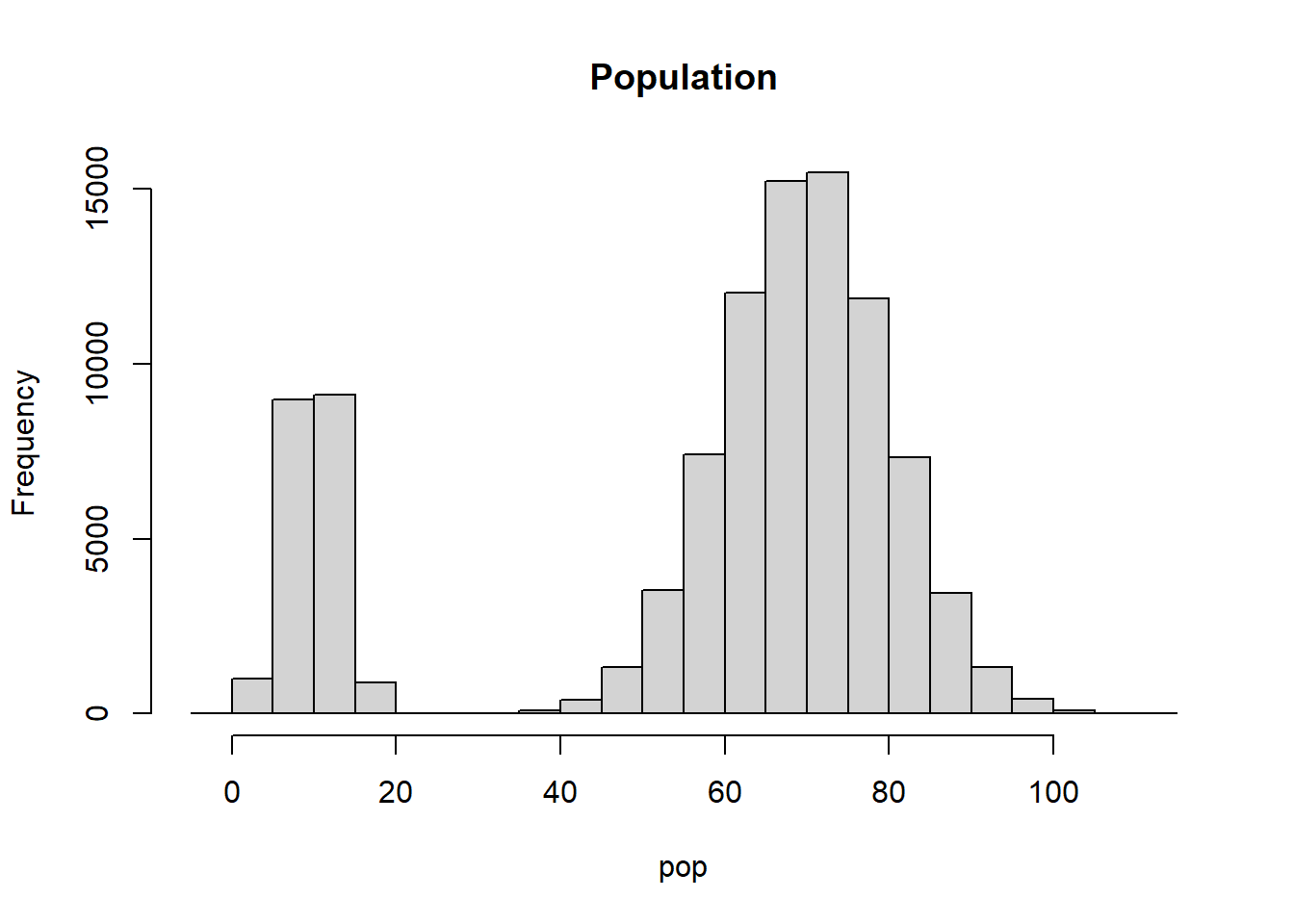
The mean and standard deviation of the population are the following:
mean(pop)[1] 57.93031sd(pop)[1] 25.62571Now we randomly select 1000 samples of size \(n=50\).
n <- 50
mats <- NULL
for(i in 1:1000){
s <- sample(pop, n, replace = TRUE)
mats <- cbind(mats, s)
}
We calculate the mean of each sample and plot the sampling distribution of the sample mean.
samplemeans <- apply(mats, 2, mean)
hist(samplemeans, main = "Sample mean")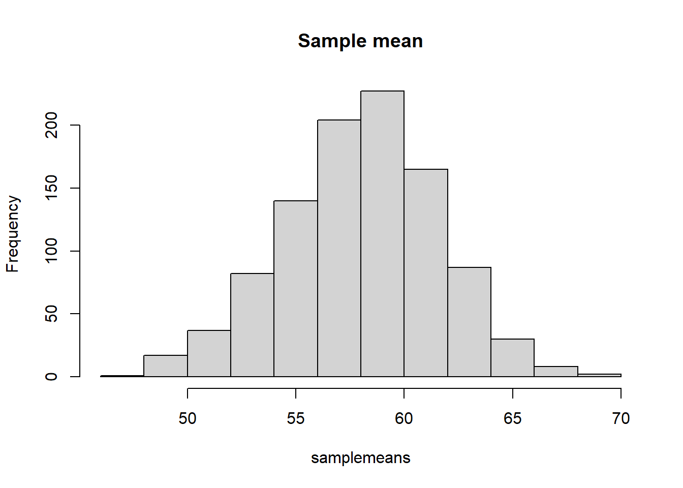
We calculate the mean and standard deviation of the sampling distribution of the sample mean and check the CLT.
Sample size \(n \geq 30\).
Sampling distribution of sample mean approximates to a normal distribution.
Mean of the sample mean is \(\mu_{\bar X} = \mu\)
mean(samplemeans)[1] 57.94416mean(pop)[1] 57.93031- Standard error (standard deviation of the sample mean) is \(\sigma_{\bar X} =\frac{\sigma}{\sqrt{n}}\)
sd(samplemeans)[1] 3.67371sd(pop)/sqrt(n)[1] 3.624022