4  Hypothesis tests

Learning objectives

• Conduct hypothesis tests and interpret results
• Identify null and alternative hypotheses
• Understand Type I and II errors
• Understand significance level
• Calculate p-value
• Conduct hypothesis tests for one mean, two means, one proportion and two proportions

4.1 What is hypothesis testing?

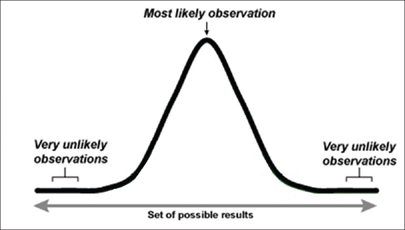
Hypothesis testing is a procedure to determine whether a claim about a population parameter is reasonable. Such a claim is called hypothesis.

• Example of research question: Does a new drug reduce cholesterol?

The alternative or research hypothesis is the research question (e.g., an alternative to the currently accepted value for the population parameter). The alternative is denoted by \(H_1\) or \(H_a\).

• \(H_1\): The new drug reduces cholesterol

The null hypothesis represents a position of “no difference” (e.g., currently accepted value for a population parameter). The null hypothesis is denoted by \(H_0\).

• \(H_0\): The new drug has no effect

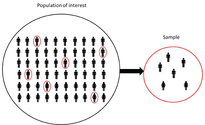
To test a hypothesis, we select a sample from the population and use measurements from the sample and probability theory to determine how well the data and the null hypothesis agree. We want to show the alternative hypothesis is reasonable (by showing there is evidence to reject the null hypothesis).

Example

• Research question we are trying to answer
  Does a new drug reduce cholesterol?

• Alternative hypothesis (investigator’s belief)
  The new drug reduces cholesterol

• Null hypothesis (no difference, hypothesis to be rejected)
  The new drug has no effect

Let \(\mu_1\) and \(\mu_2\) be the cholesterol levels obtained with and without the drug, respectively.

\(H_0: \mu_1 = \mu_2\) (Null hypothesis)

\(H_1: \mu_1 < \mu_2\) (Alternative hypothesis)

4.2 Hypothesis testing procedure

A hypothesis is tested by using the following procedure:

1. Determine the null and alternative hypotheses.

2. Select an appropriate sample from the population.

3. Assume the null hypothesis is true. Use measurements from the sample and probability theory to determine how well the data and the null agree.

4. We make one of these two decisions:

• We reject the null hypothesis if there is enough evidence in the sample to disprove it.
• We fail to reject the null hypothesis if there is not enough evidence to disprove it. Failing to reject the null does not mean null is true. We just do not have enough evidence against the null (maybe sample was not large enough or we were just unlucky).

Example

Suppose we think the mean weight of the oranges in a field is lower than 100 grams. We conduct a hypothesis test to test this claim.

1. Null and alternative hypothesis
   \(H_0\): \(\mu=100\)
   \(H_1\): \(\mu < 100\)

2. We take a sample from the population (for example, a random sample of 100 oranges).

3. We assume the null hypothesis is true, and calculate the mean weight of the oranges in the sample to decide whether to reject or fail to reject the null hypothesis.

4. We use the sample mean in the sample to make a decision.

• if the sample mean is 110 we can think we do not have evidence against the null and we fail to reject the null
• if the sample mean is 150 we can think we have some evidence against the null and we reject the null
• if the sample mean is 300 we can think we have strong evidence against the null and we reject the null

4.3 Null and alternative hypothesis

---

Null Hypothesis \(H_0\)	Alternative Hypothesis \(H_1\)
Assumed true until evidence indicates otherwise	We try to find evidence for the alternative hypothesis
“Nothing is going on”	Opposite of the null hypothesis
There is no relationship between variables being studied	There is relationship between variables being studied
A particular intervention does not make a difference/has no effect	A particular intervention makes a difference/has an effect

---

Hypothesis are written in terms of population parameters. For example, we can write hypothesis for a single mean (\(\mu\)), a single proportion (\(p\)), the difference between two independent means (\(\mu_1-\mu_2\)), and the difference between proportions (\(p_1-p_2\)).

Example

For each of the research questions below, write the null and alternative hypothesis. Remember the alternative hypothesis is the investigator’s belief and the null hypothesis denotes the hypothesis of no difference, the one we wish to reject. In general the null hypothesis contains the equal sign (\(=\)).

• Is the average monthly rent of a one-bedroom apartment in Bath less than 800 pounds?

\(H_0\): \(\mu = 800\)
\(H_1\): \(\mu < 800\)

• Is the average intelligence quotient (IQ) score of all university students higher than 100?

\(H_0\): \(\mu = 100\)
\(H_1\): \(\mu > 100\)

• Is the percent of students enrolled in Faculty of Science who identify as women different from 50%?

\(H_0: p = 0.5\)
\(H_1: p \neq 0.5\)

• Do the majority of all university students own a dog?

\(H_0: p = 0.5\)
\(H_1: p > 0.5\)

• In preschool, are the weights of boys and girls different?

\(H_0: \mu_b = \mu_g\)
\(H_1: \mu_b \neq \mu_g\)

• Is the proportion of men who smoke cigarettes different from the proportion of women who smoke cigarettes in England?

\(H_0: p_1 = p_2\)
\(H_1: p_1 \neq p_2\)

4.4 Errors in hypothesis testing

Possible outcomes for a hypothesis test:

	\(H_0\) is True	\(H_0\) is False
Reject null	Type I error (false positive)	Correct (true positive)
Fail to reject null	Correct (true negative)	Type II error (false negative)

When making a decision about a hypothesis test we can make two types of errors:

• Type I error: Reject the null hypothesis when it is true
• Type II error: Fail to reject the null hypothesis when it is false

For example, let the null hypothesis \(H_0\) be patient is not pregnant. Then,

Type I and II errors

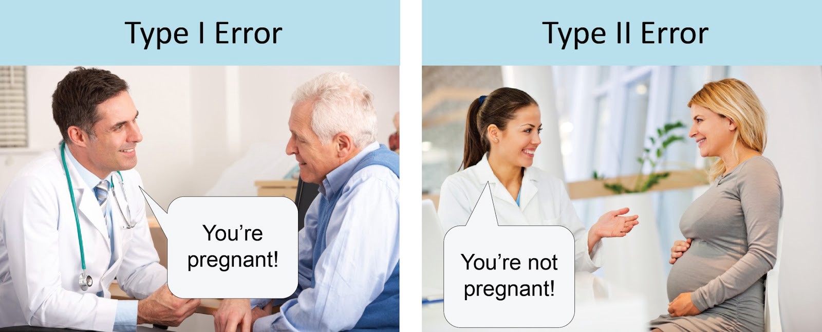
• Type I error: Reject the null hypothesis when it is true. Patient is not pregnant but we conclude he is pregnant.
• Type II error: Fail to reject the null hypothesis when it is false. Patient is pregnant but we conclude she is not pregnant.

\(\alpha\) = Probability of Type I error = P(rejecting \(H_0\) | \(H_0\) is true)

\(\beta\) = Probability of Type II error = P(failing to reject \(H_0\) | \(H_0\) is false)

• \(\alpha\) and \(\beta\) are related. As one increases, the other decreases.

• For large sample sizes, it is more likely to get significant results. Small differences may be significant so we should check if the difference is meaningful.

• A small sample size might lead to frequent Type II errors (e.g., a huge difference is needed to conclude a significant difference).

• For small sample sizes, we may fail to reject the null even though it is false.

Example

A man goes to trial where he is being tried for a murder. The hypotheses being tested are:

\(H_0\): Not guilty
\(H_1\): Guilty

What are the Type I and II errors that can be committed?

Solution

Type I error is committed if we reject \(H_0\) when it is true. In other words, the man did not kill the person but was found guilty and is punished for a crime he did not really commit.

Type II error is committed if we fail to reject \(H_0\) when it is false. In other words, if the man killed the person but was found not guilty and was not punished.

4.5 Significance level, confidence level and power of a test

4.5.1 Significance level

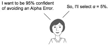
Before testing the hypothesis, we need to select the significance level (\(\alpha\)). The significance level of a test is the maximum value for the probability of Type I Error (incorrectly rejecting the null when it is true) we are willing to tolerate and still call the results statistically significant.

Typical values for \(\alpha\) are 0.05 and 0.01. If we choose \(\alpha = 0.05\), there will be a maximum of 5% chance of incorrectly rejecting the null when it is true.

4.5.2 Confidence level

The confidence level \(c\) represents how confident we are in our decision (e.g., 95%, 99%)

• \(c = 1 - \alpha\) is the confidence level
• \(\alpha= 1-c\) is the significance level

For example, if the confidence level is 95%, the significance level is \(\alpha = 1 - c = 1 - 0.95 = 0.05\).

4.5.3 Power of a test

The power of a test is the probability of correctly rejecting the null when it is false.

Power = P(reject \(H_0\) | \(H_0\) is false) = 1- P(fail to reject \(H_0\) | \(H_0\) is false) = 1 - Probability of Type II error = 1 - \(\beta\)

Power depends on the following factors:

• Significance level: Power can be increased by using a less conservative test, that is by using a greater significance level (for example \(\alpha\) equal to 0.10 instead of 0.05).
• Magnitude of the effect: There is greater power to detect large diferences.
• Sample size: As sample size increases, the sampling error decreases and the power increases.

When conducting a hypothesis test, we want both Type I and Type II errors to be small (close to 0). Unfortunately, decreasing Type I error increases Type II errors and makes it difficult to conduct tests with both small Type I errors and high power.

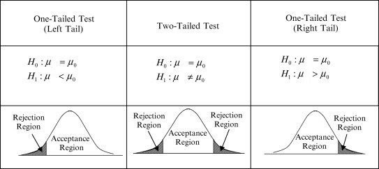
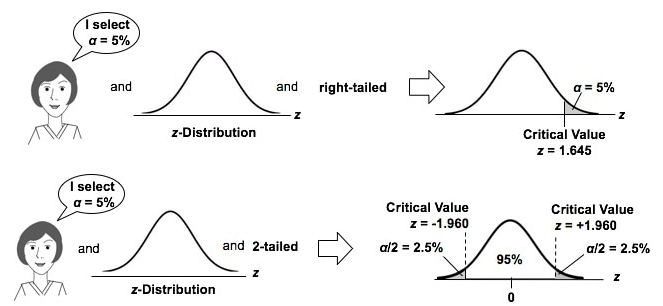
4.6 One-sided and two-sided tests

• In a one-sided (or one-tailed) test the alternative hypothesis specifies that the population parameter lies entirely above or below the value specified in \(H_0\). For example,

\(H_0: \mu=100\)
\(H_1: \mu>100\)

In practice, a one-sided test such as this is tested in the same way as the following test

\(H_0: \mu\leq100\)
\(H_1: \mu>100\)

This is because if we conclude \(\mu>100\), we must also conclude \(\mu>90\), \(\mu>80\), etc.

• In a two-sided (or two-tailed) test the alternative hypothesis specifies that the parameter can lie on either side of the value specified by \(H_0\) For example,

\(H_0: \mu=100\)
\(H_1: \mu \neq 100\)

4.7 Hypothesis test procedure

Suppose a company manufacturing computer chips claims the defective rate is 5%. Let \(p\) denote the true defective probability. We use a sample of 1000 chips from the production to determine their claim is reasonable. The proportion of defectives in the sample is 8%.

• Null and alternative hypothesis
  \(H_0: p = p_0\) (proportion of defective chips is 5%)
  \(H_1: p > p_0\) (proportion of defective chips is greater than 5%)
  where \(p_0=0.05\)

• We use a significance level \(\alpha = 0.05\) so the probability of incorrectly rejecting the null when it is true is 5%.

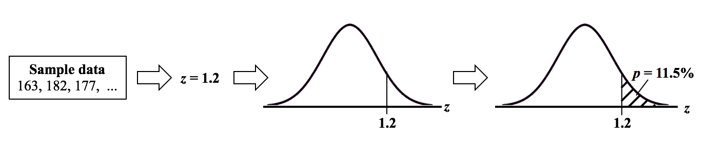
• Then we calculate the test statistic which has the general form:

\[\mbox{test statistic} = \frac{\mbox{sample statistic - null parameter}}{\mbox{standard error}}\]

The test statistic is a value calculated from a sample that summarizes the characteristics of the sample and is used to determine whether to reject or fail to reject the null hypothesis. The test statistic differs from sample to sample. The sampling distribution of the test statistic under the null hypothesis must be known so we can compare the results observed to the results expected from the null hypothesis. For example, we use test statistics with normal or t distributions. These distributions have a known area, and enable to calculate p-values (probability that tell if results are due to chance or due to hypothesis being correct).

Sampling distribution of the test statistic under the null hypothesis.

• In this example the sample statistic is the proportion of defective chips in the sample (\(\hat P\)). The test statistic \(Z\) follows a N(0, 1) distribution under the null hypothesis (this holds if we have independent observations and the number of expected successes and failures are both greater than 10).

\[Z = \frac{\hat P - p_0}{\sqrt{\frac{p_0(1-p_0)}{n}}} \sim N(0,1)\]

• The observed value of the test statistic is \(z_{obs} = \frac{0.08-0.05}{\sqrt{0.05(1-0.05)/1000}}\) = 4.35.

• Now we need to decide whether reject the null or fail to reject the null. We reject the null if the observed value of the test statistic is so extreme that it is unlikely to occur if the null is true (unlikely to occur is given by the significance level \(\alpha\)). Otherwise we fail to reject the null. There are two approaches to determine whether the test statistic is extreme and the null hypothesis should be rejected. These are the p-value approach and the critical value approach. We explain these approaches below.

• P-value approach: The p-value is the probability of obtaining a test statistic as extreme as or more extreme than the one observed in the direction of the alternative hypothesis, assuming the null hypothesis is true. We calculate the p-value as the area under the N(0,1) curve beyond the test statistic observed in the direction of the alternative hypothesis, \(P(Z > 4.35 | H_0)\). p-value = 6.8068766^{-6}. p-value < \(\alpha\). So we reject \(H_0\).

• Critical value approach: We determine the critical value by finding the value of the distribution of the test statistic under the null such that the probability of making a Type I error is the specified significance level \(\alpha = 0.05\). Critical value is the value \(z^*\) such that the probability of N(0,1) is greater than \(z^*\) is 0.05. \(z^*\) = 1.64. The value of the observed test statistic is more extreme in the direction of the alternative hypothesis than the critical value (1.64 \(<\) 4.35). So we reject \(H_0\).

4.8 Approaches to to decide whether to reject or fail to reject the null

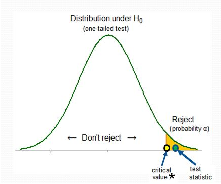
4.8.1 Critical region approach

We determine the critical value by finding the value of the distribution of the test statistic such that the probability of making a Type I error is the specified significance level \(\alpha\) (e.g., 0.05).

Then we compare the test statistic value to the critical value.

• The critical values define the boundaries of the critical or rejection region which is the set of values for which the null hypothesis is rejected. The acceptance region is the set of values that are consistent with the null hypothesis.

• If the test statistic value is more extreme in the direction of the alternative than the critical value (falls in the critical region), we reject the null hypothesis.

• If the test statistic is not more extreme in the direction of the alternative than the critical value (falls in the acceptance region), we fail to reject reject the null.

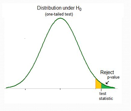
4.8.2 p-value approach

In this approach, the strength of evidence in support of the alternative hypothesis is measured by the p-value.

The p-value is the probability of obtaining a test statistic as extreme as or more extreme than the one observed in the direction of the alternative hypothesis, assuming the null hypothesis is true.

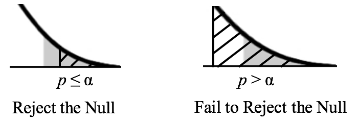
We compare the p-value to the significance level \(\alpha\) and decide whether to reject or fail to reject the null.

• If p-value < \(\alpha\), we reject the null hypothesis
• If p-value \(\geq \alpha\), we fail to reject the null hypothesis

4.8.2.1 Calculate p-value

The p-value is the probability of observing a test statistic as extreme as or more extreme than the one observed in the direction of the alternative hypothesis, assuming that the null hypothesis is true.

To calculate the p-value we compute the test statistic value using the sample data, and calculate the area under the test statistic distribution curve beyond the test statistic value.

4.8.2.2 Compare p-value and \(\alpha\)

• If p-value is small (p-value \(<\) \(\alpha\)) this indicates that we had little chance of getting our data if the null hypothesis is true. So we reject the null. We can say: The test result is statistically significant. We conclude there is evidence against the null hypothesis. The data provide convincing evidence for the alternative hypothesis.

• If p-value is big ( p-value \(\geq\) \(\alpha\)) this indicates that there is reasonable chance of getting our data if the null hypothesis is true. So we fail to reject the null.
  We can say: The test result is not statistically significant. We conclude there is not sufficient evidence against the null hypothesis. The data do not provide convincing evidence for the alternative hypothesis. (If we fail to reject the null, this does not mean the null is true, it only means we do not have sufficient evidence against the null).

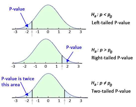
4.8.2.3 p-values in one- and two- tailed tests

• In left-tailed tests, the p-value is calculated as the area under the test statistic distribution curve to the left of the test statistic.

• In right-tailed tests, the p-value is calculated as the area under the test statistic distribution curve to the right of the test statistic.

• In two-tailed tests, the p-value is calculated by using the symmetry of the test distribution curve. We find the p-value for a one-sided test and double it.

4.9 Examples

4.9.1 Steps in hypothesis testing

1. State the null and alternative hypotheses.
   The alternative hypothesis is the investigator’s belief and the null hypothesis denotes the hypothesis of no difference, the one we wish to reject. The null hypothesis contains the equal sign (\(=\)).

2. Choose the significance level (maximum value for the probability of incorrectly rejecting the null when it is true we are willing to tolerate)
   Usually \(\alpha = 0.05\)

3. Calculate the test statistic.
   \(\mbox{test statistic} = \frac{\mbox{sample statistic - null parameter}}{\mbox{standard error}}\)

4. Find the p-value for the observed data.
   The p-value is the probability of obtaining a test statistic as extreme as or more extreme than the one observed in the direction of the alternative hypothesis, assuming the null hypothesis is true.

5. Make one of these two decisions and state a conclusion.

• If p-value < \(\alpha\), we reject the null hypothesis
• If p-value \(\geq \alpha\), we fail to reject the null hypothesis

Below we give examples of the following tests:

	Population parameter	Sample statistic	Test statistic
One Mean	\(\mu\)	\(\bar X\)	\(T=\frac{\bar X - \mu_0}{S/\sqrt{n}} \sim t(n-1)\)
One Proportion	\(p\)	\(\hat P\)	\(Z = \frac{\hat P - p_0}{\sqrt{\frac{p_0(1-p_0)}{n}}} \sim N(0,1)\)
Difference in two proportions	\(p_1 - p_2\)	\(\hat P_1 - \hat P_2\)	\(Z = \frac{(\hat P_1 - \hat P_2)-0}{\sqrt{\frac{\hat P (1-\hat P)}{n_1} + \frac{\hat P (1-\hat P)}{n_2}}} \sim N(0,1)\)
Difference in two means (independent samples)	\(\mu_1 - \mu_2\)	\(\bar X_1 - \bar X_2\)	\(T = \frac{(\bar X_1 - \bar X_2) - 0}{\sqrt{\frac{S_1^2}{n_1}+\frac{S_2^2}{n_2} }} \sim t(min(n_1-1,n_2-1))\)
Difference in two means (paired samples)	\(\mu_{diff}\)	\(\bar X_{diff}\)	\(T= \frac{\bar X_{diff}}{S_{diff}/\sqrt{n}} \sim t(n-1)\)

4.9.2 One mean

https://ismayc.github.io/moderndiver-book/B-appendixB.html#one-mean

The National Survey of Family Growth conducted by the Centers for Disease Control gathers information on family life, marriage and divorce, pregnancy, infertility, use of contraception, and men’s and women’s health. One of the variables collected on this survey is the age at first marriage. 5,534 randomly sampled US women between 2006 and 2010 completed the survey. The women sampled here had been married at least once. The sample mean is 23.44 and the standard deviation 4.72. Do we have evidence that the mean age of first marriage for all US women from 2006 to 2010 is greater than 23 years?

Data: Sample size \(n=5534\), sample mean \(\bar x_{obs}=23.44\), standard deviation \(s=4.72\).

1. Null and alternative hypotheses

\(H_0: \mu \leq 23\)
\(H_1: \mu > 23\)

(\(\mu_0\) is 23)

Guess about statistical significance

We want to see how likely is it to have observed a sample mean of \(\bar x_{obs}=23.44\) or more extreme assuming that the population mean is 23 (assuming the null is true). They seem to be quite close, but we have a large sample size. Let’s guess that the large sample size will lead us to reject this practically small difference.

2. Choose \(\alpha\)

\(\alpha = 0.05\)

3. Test statistic

A good guess to estimate the population mean \(\mu\) is the sample mean \(\bar X\). Assuming the null is true, we can standardize this original test statistic \(\bar X\) into a \(T\) statistic that follows a \(t\) distribution with degrees of freedom equal df\(=n-1\).

\[T=\frac{\bar X - \mu_0}{S/\sqrt{n}} \sim t(n-1)\]

Assumptions: Independent observations (random sample) and normality (normality or sample size \(\geq\) 30)

n <- 5534
barx <- 23.44
s <- 4.72
t <- (barx-23)/(s/sqrt(n))
t

[1] 6.934741

4. p-value

Probability of observing a test statistic of 6.93 or more extreme in the t-distribution.

df <- n-1
1 - pt(t, df = df)

[1] 2.267297e-12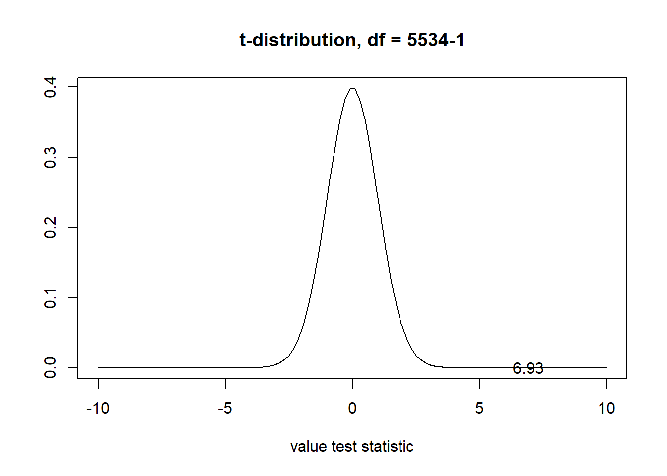

5. Decision

p-value < \(\alpha\), we reject the null. We have found evidence the mean age of first marriage is greater than 23.

4.9.3 One proportion

https://ismayc.github.io/moderndiver-book/B-appendixB.html#one-proportion

The CEO of a large electric utility claims that 80 percent of his 1,000,000 customers are satisfied with the service they receive. To test this claim, the local newspaper surveyed 100 customers, using simple random sampling. 73 were satisfied and the remaining were unsatisfied. Based on these findings from the sample, can we reject the CEO’s hypothesis that 80% of the customers are satisfied?

Data: Sample size \(n=100\), sample proportion \(\hat p_{obs}=0.73\)

1. Null and alternative hypotheses

\(H_0: p = 0.80\)
\(H_1: p \neq 0.80\)

(\(p_0=0.80\))

Guess about statistical significance

We want to see if the sample proportion 0.73 is statistically different from \(p_0=0.8\). They seem to be close and the sample size is not big (\(n=100\)). We may guess that we do not have evidence to reject the null hypothesis.

2. Significance level

\(\alpha = 0.05\)

3. Test statistic

A good guess to estimate the population proportion \(p\) is the sample proportion \(\hat P\). Assuming the null is true, we can standardize the original test statistic \(\hat P\) into a \(Z\) statistic that follows a \(N(0,1)\).

\[Z = \frac{\hat P - p_0}{\sqrt{\frac{p_0(1-p_0)}{n}}} \sim N(0,1)\]

Assumptions: Independent observations (random sample) and number of expected successes (73) and failures (27) are both greater than 10

n <- 100
p_hat <- 0.73
p0 <- 0.8
z <- (p_hat-p0)/sqrt((p0*(1-p0))/n)
z

[1] -1.75

4. p-value

Probability of observing a test statistic value of -1.75 or more extreme (in both directions) in the null distribution.

2*pnorm(z)

[1] 0.08011831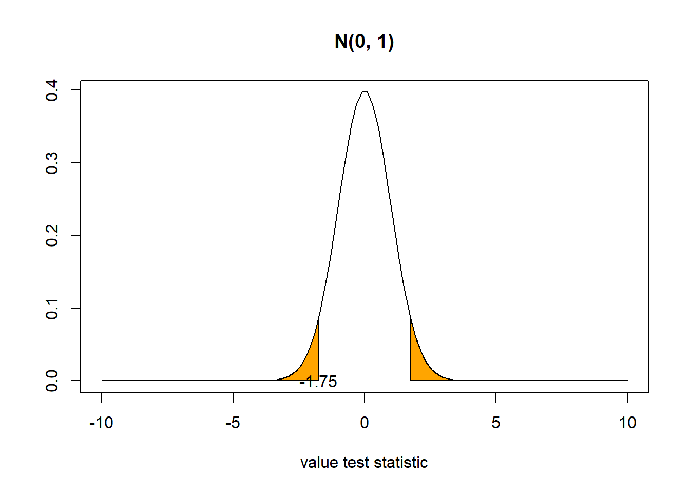

5. Decision

p-value > \(\alpha\), we fail to reject the null. We do not find enough evidence to reject the null.

4.9.4 Two proportions

https://ismayc.github.io/moderndiver-book/B-appendixB.html#two-proportions

A 2010 survey asked 827 randomly sampled registered voters in California “Do you support? Or do you oppose? Drilling for oil and natural gas off the Coast of California? Or do you not know enough to say?” Conduct a hypothesis test to determine if the data provide strong evidence that the proportion of college graduates who do not have an opinion on this issue is different than that of non-college graduates.

Data

Sample size \(n=827\)

	no opinion	opinion
college	131	258
no college	104	334

1. Null and alternative hypotheses

\(H_0: p_c = p_{nc}\)
\(H_1: p_c \neq p_{nc}\)

or

\(H_0: p_c - p_{nc} = 0\)
\(H_1: p_c - p_{nc} \neq 0\)

Guess about statistical significance

We want to know if there is a statistically significant difference between the college proportion and the non-college proportion. The proportions are close:

• college proportion 131/(131+258) = 0.33
• non-college proportion 104/(104+334) = 0.23

We could guess there is not evidence to reject the null.

2. Set \(\alpha\)

\(\alpha = 0.05\)

3. Test statistic

We are interested in seeing if the observed difference in sample proportions corresponding to no opinion (\(\hat p_{1obs} - \hat p_{2obs}\)) is statistically different from 0. Assuming the null is true, we can use the standard normal distribution to standardize the difference in sample proportions

\[Z = \frac{(\hat P_1 - \hat P_2)-0}{\sqrt{\frac{\hat P (1-\hat P)}{n_1} + \frac{\hat P (1-\hat P)}{n_2}}} \sim N(0,1)\]

where \(\hat P = \frac{\mbox{total number of successes}}{\mbox{total number of cases}}\)

Assumptions: Independent observations (random sample) and number of pooled successes and pooled failures at least 10 for each group (\(n \hat p \geq 10\) and \(n (1 - \hat p) \geq 10\)). Pooled success rate: \(\hat p\) = (131+104)/827 = 0.28, \(1-\hat p\) = 0.72. \(\hat p \times (131+258) = 108.92\), \((1-\hat p) \times (131+258) = 280.08\), \(\hat p \times (104+334) = 122.64\), \((1-\hat p) \times (104+334) = 315.36\)

n1 <- 131+258
p1 <- 131/(131+258)
n2 <- 104+334
p2 <- 104/(104+334)
phat <- (131+104)/(131+258+104+334)
z <- (p1-p2)/sqrt(phat*(1-phat)/n1 + phat*(1-phat)/n2)
z

[1] 3.160806

4. p-value

Probability observing a test statistic equal to 3.16 or more extreme (in both directions) when the null is true.

2 * (1-pnorm(z))

[1] 0.001573334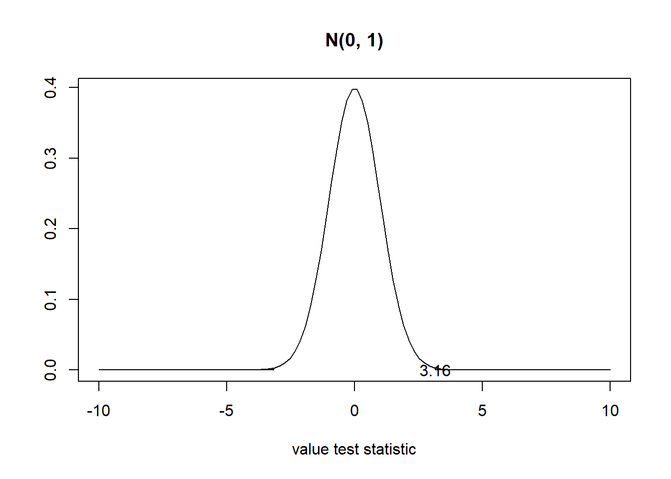

5. Decision

p-value < \(\alpha\), we reject the null. There is evidence proportions are different. We do have evidence to suggest that there is a dependency between college graduation and position on offshore drilling for Californians. Our initial guess was wrong!

4.9.5 Two means (independent samples)

https://ismayc.github.io/moderndiver-book/B-appendixB.html#two-means-independent-samples

Average income varies from one region of the country to another, and it often reflects both lifestyles and regional living expenses. Suppose a new graduate is considering a job in two locations, Cleveland, OH and Sacramento, CA, and he wants to see whether the average income in one of these cities is higher than the other. He would like to conduct a hypothesis test based on two randomly selected samples from the 2000 Census.

Data:
Ohio: \(n_1= 212\), \(\bar x_1= 27467\), \(s_1= 27681\)
Cleveland: \(n_2= 175\), \(\bar x_2= 32428\), \(s_2= 35774\)

1. Null and alternative hypotheses

\(H_0: \mu_1 = \mu_2\)
\(H_1: \mu_1 \neq \mu_2\)

or

\(H_0: \mu_1- \mu_2 = 0\)
\(H_1: \mu_1 - \mu_2 \neq 0\)

Guess about statistical significance

We want to see if the average income in Cleveland is statistically different than the average income in Sacramento. In the sample we observe

Ohio: \(n_1= 212\), \(\bar x_1= 27467\), \(s_1= 27681\)
Cleveland: \(n_2= 175\), \(\bar x_2= 32428\), \(s_2= 35774\)

The distributions seem similar. We guess there is not enough evidence to support the average incomes are different.

2. Set \(\alpha\)

\(\alpha = 0.05\)

3. Test statistic

We wish to see if the observed difference in sample means is statistically different than 0. Assuming the null is true, we can use the \(t\) distribution to standardize the difference in the sample means \(\bar X_1 - \bar X_2\).

\[T = \frac{(\bar X_1 - \bar X_2) - 0}{\sqrt{\frac{S_1^2}{n_1}+\frac{S_2^2}{n_2} }} \sim t(min(n_1-1,n_2-1))\] Assumptions: Independent observations and normality (distribution normal or samples sizes \(\geq\) 30)

n1 <- 212
x1 <- 27467
s1 <- 27681

n2 <- 175
x2 <- 32428
s2 <- 35774

t <- (x1-x2)/sqrt(s1^2/n1+s2^2/n2)
t

[1] -1.500762

4. p-value

Probability of observing a value of the test statistic equal -1.5 to or more extreme (in both directions) assuming the null is true

df <- min(n1-1, n2-1) # 174
2*(pt(t, df))

[1] 0.1352296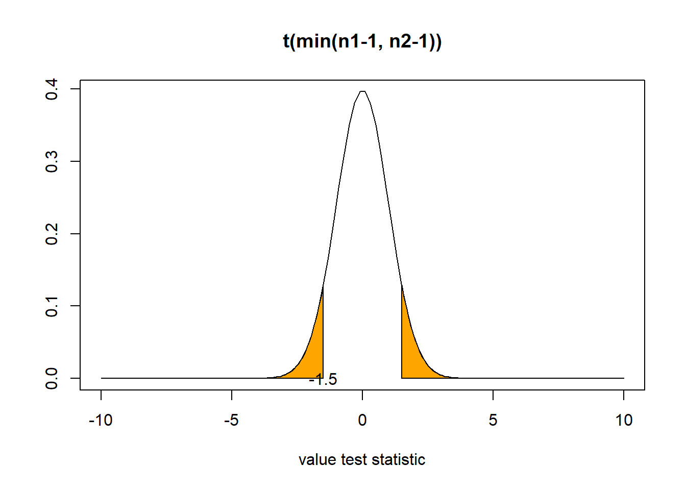

5. Decision

p-value > \(\alpha\). We fail to reject the null. There is not enough evidence to reject the null.

Note

Note that if we assume that the two samples are drawn from populations with identical population variances. The test statistic is calculated as

\[T = \frac{(\bar X_1 - \bar X_2) - 0}{\sqrt{\frac{S_p^2}{n_1}+\frac{S_p^2}{n_2} }} \sim t(n_1+n_2-2)\]

where \(S_p^2\) is an estimator of the pooled variance of the two groups.

\[S_p^2 = \frac{(n_1-1)S_1^2 + (n_2-1)S_2^2 }{n_1+n_2-2}\]

4.9.6 Two means (paired samples)

https://ismayc.github.io/moderndiver-book/B-appendixB.html#two-means-paired-samples

We can also conduct hypothesis tests with paired data. For example, we can have before-and-after measurements for a sample of people and may want to analyze the differences using a paired sample t-test.

If data are paired, and the response variable is quantitative, then the outcome of interest is the mean difference. In a population this is \(\mu_{diff}\) and in a sample \(\bar x_{diff}\). We would first compute the differences for each case, then treat those differences as if they are the variable of interest and conduct a single sample mean test.

Trace metals in drinking water affect the flavor and an unusually high concentration can pose a health hazard. Ten pairs of data were taken measuring zinc concentration in bottom water and surface water at 10 randomly selected locations on a stretch of river. Do the data suggest that the true average concentration in the surface water is smaller than that of bottom water?

Data: \(n=10\), \(\bar x_{diff}\) = -0.08, sd =0.052

1. Null and alternative hypotheses

\(\mu_1\): average concentration in surface water
\(\mu_2\): average concentration in bottom water

\(H_0: \mu_1 \geq \mu_2\)
\(H_1: \mu_1 < \mu_2\)

or

\(H_0: \mu_{diff} \geq 0\)
\(H_0: \mu_{diff} < 0\)

\(\mu_{diff}\) is the mean difference in concentration for surface water minus bottom water.

Guess about statitical significance.

We want to know if there is a statistical significant difference in concentration between surface water and bottom water.

We want to know if the sample paired mean difference of -0.08 is statistically lower than 0. The difference seems close to 0 but the sample size is small (\(n=10\)). We guess there is not evidence to reject the null.

2. Set \(\alpha\)

\(\alpha = 0.05\)

3. Test statistic

An estimate for the population mean difference \(\mu_{diff}\) is the sample mean difference \(\bar X_{diff}\). Assuming the null is true, we can standardize the original test statistic \(\bar X_{diff}\) into a \(T\) statistic that follows a \(t\) distribution with degrees of freedom df = \(n-1\).

\[T= \frac{\bar X_{diff}}{S_{diff}/\sqrt{n}} \sim t(n-1)\] Assumptions: Independent observations (observations among pairs are idependent) and normality (distribution population of differences is normal or pairs \(\geq\) 30). Here we also only have 10 pairs which is fewer than the 30 needed. We would need to check data are normal!

n <- 10
xdiff <- -0.08
sdiff <- 0.052
t <- xdiff/(sdiff/sqrt(n))
t

[1] -4.865043

4. p-value

Probability of obtainig a test statistic equal to -4.86 or lower under the null hypothesis

df <- n-1
pt(t, df)

[1] 0.0004447997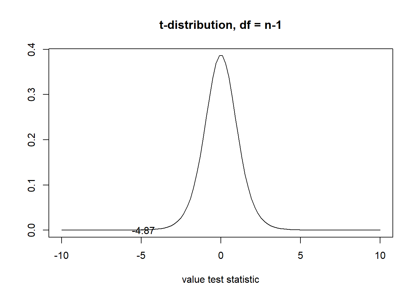

5. Decision

p-value < \(\alpha\), we reject the null hypothesis. We have evidence that the mean concentration in the surface water is lower than in the bottom water.