3 Confidence intervals

Learning objectives

Calculate and interpret confidence intervals
Confidence intervals for a population proportion
Confidence intervals for a population mean

4 Statistical inference

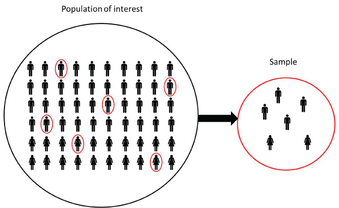
In statistical inference we are interested in learning some quantity representing some parameter of a population. Population is large and we cannot examine all the values in the population directly. Therefore, to learn about the population parameter we take a sample of size $n$ from the population and use the information in the samples to draw conclusions about the population.

We can estimate population parameters by providing point estimates (single values) and interval estimates (range of values).

For example, the proportion of the population with a given characteristic ($p$) can be estimated with the sample proportion ($\hat p$) (e.g., proportion of smokers).
The mean of a population characteristic $\mu$ can be estimated with the sample mean ($\bar x$) (e.g., mean height of population).
A confidence interval provides a range of plausible values for the population parameter. Values outside the confidence interval are unlikely to be the true population parameter.
A point estimate gives the most likely value of the population parameter. A confidence interval is a range of values that is likely to contain the population parameter, and represents the precision of the point estimate.
If we take a different sample, the value of the point estimate and the confidence interval will change.

5 Confidence interval

A confidence interval for an unknown population parameter provides a range of plausible values where we may find the true population parameter.

A $(c \times 100)$% confidence interval for a population parameter $\mu$ based on observations $X=(X_1, \ldots, X_n)$ is a pair of statistics $A(X)$ and $B(X)$ such that

\[P(A(X)\leq \mu \leq B(X))=c\] Note the values of $A(X)$ and $B(X)$ change with each sample.

Confidence level $c = 1 - \alpha$ and significance level $\alpha = 1- c$.

Interpretation:

If we construct a 95% confidence interval for a population parameter, we are 95% confident that the population parameter is within the interval.
If we take many samples of size $n$ from the population, and calculate the 95% CIs for each sample, then 95% of these CIs will contain the true population parameter.

Construct a confidence interval

Select a confidence level $c$ that describes the uncertainty of the sampling method. Common confidence levels are 95% and 90%
Identify a sample statistic that is used to estimate the population parameter. For example, the sample mean ($\bar X$) to estimate the population mean ($\mu$), or the sample proportion ($\hat P$) to estimate the population proportion ($p$)
Identify the sampling distribution of the sample statistic and the standard error (SE)
Specify the confidence interval as

\[\mbox{sample statistic $\pm$ critical value $\times$ SE}\]

Sample statistic (e.g., $\bar X$, $\hat P$)
Critical value (e.g., $z^*$, $t^*(n-1)$). The critical is the value such that the area between -(critical value) and (critical value) of the sampling distribution corresponds to the confidence level $c$. The critical value measures the number of SE to be added and subtracted from the sample statistic in order to achieve the desired confidence level
Standard error SE is the standard deviation of the sampling distribution of the sample statistic
The margin of error is the critical value $\times$ SE

6 Confidence interval for a proportion

A $(1-\alpha) \times 100$% confidence interval for the population proportion $p$ is

\[\hat P \pm z^* \times SE = \hat P \pm z^* \times \sqrt{\hat P(1-\hat P)/n}\]

where $z^*$ is the value such that $\alpha/2$ of the probability in the standard normal distribution is below $z^*$

The conditions required to construct the confidence interval are

Sample observations are independent (e.g., are from a random sample)
There are at least 10 successes and 10 failures in the sample (i.e., $n \hat p \geq 10$ and $n(1- \hat p)\geq 10$)

For example, a 95% confidence interval for a proportion can be calculated as

\[(\hat P - 1.96 \times \sqrt{\hat P(1-\hat P)/n},\ \hat P + 1.96 \times \sqrt{\hat P(1-\hat P)/n})\]

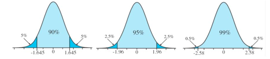
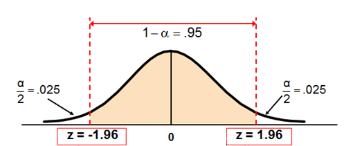
We select $z^*$ so that the area between $-z^*$ and $z^*$ in the standard normal distribution, N(0, 1), corresponds to the confidence level $c=1-\alpha$. $z^*$ is the value such that $\alpha/2$ of the probability in the standard normal distribution is below $z^*$.

For a 90% confidence interval, $c=0.90$, $\alpha=0.10$, $z^*$ = 1.64
For a 95% confidence interval, $c=0.95$, $\alpha=0.05$, $z^*$ = 1.96
For a 99% confidence interval, $c=0.99$, $\alpha=0.01$, $z^*$ = 2.57

6.1 Central Limit Theorem for a proportion

The sampling distribution of the sample proportion $\hat P$ is approximately normal with mean the population proportion $p$ and standard error SE = $\sqrt{\frac{p(1-p)}{n}}$ \[\hat P \sim N\left(p, \sqrt{\frac{p(1-p)}{n}}\right)\] when the following conditions are satisfied:

Sample observations are independent (e.g., are from a random sample)
Sample size is sufficiently large such that we expect to see at least 10 successes and 10 failures in the sample (i.e., $np \geq 10$ and $n(1-p)\geq 10$)

Proof:

$\hat P$ is the proportion of successes in $n$ trials. So $\hat P$ is equal to $Y/n$ where $Y \sim Binomial(n, p)$.

$Y$ can be expressed as the sum of $n$ independent, identically distributed Bernoulli random variables, \[Y = \sum_{i=1}^n X_i\] \[\mbox{with } X_i \sim Ber(p),\ E[X_i]=p,\ Var[X_i]=p(1-p).\]

The Central Limit Theorem says that when we collect a sufficiently large sample of $n$ independent observations, the sampling distribution of the sample mean $\bar X \sim N(\mu, \frac{\sigma}{\sqrt{n}})$. Thus,

\[\hat P = \frac{\sum_{i=1}^n X_i}{n} \sim N\left(p, \sqrt{\frac{p(1-p)}{n}}\right)\]

6.2 Confidence interval for a proportion

We can standardize $\hat P$ \[Z = \frac{\hat P - p}{\sqrt{p(1-p)/n}} \sim N(0, 1)\]

\[P(-1.96 \leq \frac{\hat P - p}{\sqrt{\hat P(1-\hat P)/n}} \leq 1.96) = 0.95\]

The probability is 95% that $\hat P$ is within 1.96 standard errors of its mean.

\[P(\hat P -1.96 \times {\sqrt{\hat P(1-\hat P)/n}} \leq p \leq \hat P + 1.96 \times {\sqrt{\hat P(1-\hat P)/n}}) = 0.95\]

A $(1-\alpha) \times 100$% confidence interval for $p$ is \[(\hat P -z^* \times {\sqrt{\hat P(1-\hat P)/n}},\ \hat P + z^* \times {\sqrt{\hat P(1-\hat P)/n}})\]

where $z^*$ quantile $\alpha/2$, value such $\alpha/2$ of the probability in the N(0,1) distribution is below $z^*$.

6.3 Example. Confidence interval for a proportion

In a random sample of 40 students, 24 said they bought a copy of the textbook. Estimate the proportion of all students who bought the book and give a 95% confidence interval.

Solution \[\hat p \pm z^* \times SE = \hat p \pm z^* \times \sqrt{\hat p(1-\hat p)/n}\] Assumptions:

Sample observations independent (random sample)
At least 10 successes ($24>10$) and 10 failures ($40-24=16>10$)

Sample statistic: $\hat p = 24/40 = 0.6$

Critical value: $z^* = -1.96$
($\alpha/2$ of the probability in $N(0,1)$ is below $z^*$)

qnorm(0.025)

[1] -1.959964

$\hat p \pm z^* \times SE = \hat p \pm z^* \times \sqrt{\hat p(1-\hat p)/n} = 0.6 \pm 1.96 \times \sqrt{ 0.6(1-0.6)/40} = (0.448, 0.752)$

An estimate of the proportion of students who bought the book is 60%.

We are 95% confident that the proportion of students is between 44.8% and 75.2%.

6.4 Example. Confidence interval for a proportion

A random sample of 826 people living in UK was surveyed to better understand their political preferences. 70% of the responses supported the political party A. Calculate a 95% confidence interval for the proportion of people that support the political party A.

Solution \[\hat p \pm z^* \times SE = \hat p \pm z^* \times \sqrt{\hat p(1-\hat p)/n}\]

Assumptions:

Observations are independent (they are from a random sample)
In the sample at least 10 support ($n \hat p = 826 \times 0.70 = 578 \geq 10$ and at least 10 do not support ($n(1- \hat p) = 826 \times (1-0.70) = 248 \geq 10$)

Sample statistic: $\hat p = 24/40 = 0.70$

Critical value: $z^* = -1.96$
($\alpha/2=0.05/2$ of the probability in $N(0,1)$ is below $z^*$)

qnorm(0.025)

[1] -1.959964

$\hat p \pm z^* \times SE = \hat p \pm z^* \times \sqrt{\hat p(1-\hat p)/n} = 0.70 \pm 1.96 \times 0.016 = (0.669, 0.731)$

We are 95% confident that the true proportion of people who support political party A is between 0.669 and 0.731.

7 Confidence interval for a mean

A $(1-\alpha) \times 100$% confidence interval for the population mean $\mu$ is

\[\bar X \pm t_{n-1}^* \times SE = \bar X \pm t_{n-1}^* \times \frac{S}{\sqrt{n}}\] where $t^*_{n-1}$ is the value such that $\alpha/2$ of the probability in the $t(n-1)$ distribution is below $t^*_{n-1}$

The conditions required to construct the confidence interval are

Sample observations are independent.
Sample observations come from a normally distributed population.

When the population standard deviation is known we construct the confidence interval as follows

\[\bar X \pm z^* \times SE = \bar X \pm z^* \times \frac{\sigma}{\sqrt{n}}\]

where $z^*$ is the value such that $\alpha/2$ of the probability in the standard normal distribution is below $z^*$

For example, a 95% confidence interval for the population mean when $\sigma$ is known can be calculated as

\[(\bar X - 1.96 \times \frac{\sigma}{\sqrt{n}},\ \bar X + 1.96 \times \frac{\sigma}{\sqrt{n}})\]

7.1 Central Limit Theorem for the mean

The sampling distribution of $\bar X$ is approximately normal with mean $\mu$ and standard error SE = $\frac{\sigma}{\sqrt{n}}$

\[\bar X \sim N\left(\mu, \frac{\sigma}{\sqrt{n}}\right)\]

when the following conditions are satisfied:

Sample observations are independent (for example, sample is a random sample from the population).
Sample observations come from a normally distributed population or $n \geq 30$

If $n < 30$ and there are not clear outliers in the data, we typically assume data come from a normal distribution.
If $n \geq 30$, we typically assume the sampling distribution of $\bar X$ is normal, even if the underlying distribution of observations are not.

7.2 Confidence interval for a mean

We can standardize $\bar X$ \[Z = \frac{\bar X - \mu}{\sigma/\sqrt{n}} \sim N(0, 1)\]

\[P(-1.96 \leq \frac{\bar X - \mu}{\sigma/\sqrt{n}} \leq 1.96) = 0.95\]

The probability is about 95% that $\bar X$ is within 1.96 standard errors of its mean.

\[P(\bar X -1.96 \times \frac{\sigma}{\sqrt{n}} \leq \ \mu \leq \bar X + 1.96 \times \frac{\sigma}{\sqrt{n}}) = 0.95\] A $(1-\alpha) \times 100$% confidence interval for $\mu$ is \[(\bar X -z^* \times \frac{\sigma}{\sqrt{n}} , \bar X + z^* \times \frac{\sigma}{\sqrt{n}})\]

where $z^*$ quantile $\alpha/2$, value such $\alpha/2$ of the probability in the N(0,1) distribution is below $z^*$.

7.3 Confidence interval for a mean when $\sigma$ is not known

In practice, we cannot directly calculate the standard error for $\bar X$ since we do not know the population standard deviation, $\sigma$. When the population standard deviation $\sigma$ is not known, we approximate $\sigma$ with the sample standard deviation $S$: \[SE = \frac{\sigma}{\sqrt{n}} \approx \frac{S}{\sqrt{n}}\]

When the sample size is big we can accurately estimate $\sigma$ with $S$. However, the estimate is less precise with smaller samples and this leads to problems when using the normal distribution to model $\bar X$. Therefore we use the t distribution with $n-1$ degrees of freedom.

\[T = \frac{\bar X - \mu}{S/\sqrt{n}} \sim t(n-1)\]

A $(1-\alpha) \times 100$% confidence interval for $\mu$ is \[(\bar X - t^*_{n-1} \frac{S}{\sqrt{n}},\ \bar X + t^*_{n-1} \frac{S}{\sqrt{n}})\]

where $t^*_{n-1}$ quantile $\alpha/2$, value such $\alpha/2$ of the probability in the t(n-1) distribution is below $t^*_{n-1}$.

In general, we construct a confidence interval for the population mean by using a t distribution $n-1$ degrees of freedom. Note that when we have a large number of observations, the degrees of freedom of the t distribution will be large and the t distribution will look like the standard normal distribution (when the degrees of freedom is greater than 30, the t-distribution is nearly indistinguishable from the normal distribution).

7.4 Example. Confidence interval for a mean

In a class survey, students are asked how many hours they sleep per night. In a sample of 52 students, the mean was 5.77 hours with a standard deviation of 1.572 hours. Construct a 95% confidence interval for the mean number of hours slept per night in the population from which this sample was drawn.

Solution

$\sigma$ is unknown, we use $s$ and a t distribution with $n-1=52-1$ df \[\bar x \pm t^*_{51} \times SE = \bar x - t^*_{51} \times \frac{s}{\sqrt{n}}\]

Assumptions:

We assume data are independent
We assume data are normal

Sample statistic: $\bar x = 5.77$

Critical value: $t^*_{51}= -2.01$
($\alpha/2=0.05/2$ of the probability in t(51) is below $t^*_{51}$)

qt(0.025, 51)

[1] -2.007584

$\bar x \pm t^*_{51} \times SE = \bar x \pm t^*_{51} \times \frac{s}{\sqrt{n}} = 5.77 \pm 2.01 \times \frac{1.572}{\sqrt{52}} = (5.33, 6.21)$.

We are 95% confident the population mean is between 5.33 and 6.21 hours.

7.5 Example. Confidence interval for a mean

Elevated mercury concentrations are an important problem for both dolphins and other animals who occasionally eat them. Calculate a 95% CI for the average mercury content in dolphins using a sample of 19 dolphins in Japan. In the sample, $n=19$, $\bar x = 4.4$, $s = 2.3$, minimum $= 1.7$ and maximum $= 9.2$ $\mu$g/wet gram (micrograms of mercury per wet gram of muscle).

Solution

$\sigma$ is unknown, we use $s$ and a t distribution with $n-1=19-1$ df \[\bar x \pm t^*_{18} \times SE = \bar x \pm t^*_{18} \times \frac{s}{\sqrt{n}}\]

Assumptions:

Independence seems reasonable because observations come from a random sample.
Normality seems reasonable because there are not clear outliers (all observations are within 2.5 standard deviations of the mean).

Sample statistic: $\bar x = 4.4$

Critical value: $t^*_{18} = -2.10$
($\alpha/2=0.05/2$ of the probability in the t(18) distribution is below $t^*_{18}$)

qt(0.025, 18)

[1] -2.100922

$\bar x \pm t^*_{18} \times SE = \bar x \pm t^*_{18} \times \frac{s}{\sqrt{n}} = 4.4 \pm 2.10 \times \frac{2.3}{\sqrt{19}} = (3.29, 5.51)$

We are 95% confident the average mercury content in dolphins is between 3.29 and 5.51 $\mu$g/wet gram.

8 Interpretation of a confidence interval

A 95% CI for a population parameter denotes we are 95% confident the population parameter lies within the interval.

It is incorrect to say that there is a probability equal to 0.95 that the population parameter lies within the interval because the population parameter is a constant value and therefore the probability that the population parameter lies within the confidence interval is 0 or 1.

The interpretation of a 95% CI constructed using a sample of size $n$ is that if we take many samples of size $n$ from the population, and calculate the 95% CIs for each sample, then we would expect 95% of these CI to contain the value of the population parameter.

We can illustrate this by means of a simulation. Specifically, we consider a population and calculate many 95% CIs for the population mean. Then we observe 95% of the CIs contain the population mean.

Let us consider a population of size $N=100000$

population <- rnorm(100000)
population_mean <- mean(population)
population_mean

[1] -0.001880581

The population mean is -0.0018806. Now we take sample of size $n=100$ and calculate a 95% CI for the population mean.

(quant <- qt(1 - 0.05/2, 100-1))

[1] 1.984217

sample1 <- sample(population, 100)
ll <- mean(sample1) - quant * (sd(sample1)/sqrt(length(sample1)))
ul <- mean(sample1) + quant * (sd(sample1)/sqrt(length(sample1)))
c(ll, ul)

[1] -0.2479456  0.1410243

We are 95% confident that the population mean is within -0.2479456 and 0.1410243.

The 95% CI is constructed in a way such that if we take many samples of size $n=100$ from the population and calculate 95% CIs for each of them, 95% of the intervals will contain the population mean. We can see this by means of a simulation. First, we take $M=1000$ samples of size $n=100$ from the population.

n <- 100  # sample size
M <- 1000 # number of samples
samples <- matrix(NA, nrow = M, ncol = n) # matrix with the samples
for(m in 1:M){
samples[m, ] <- sample(population, n)
}

Then we calculate 95% CI for each sample.

ll <- apply(samples, 1,
FUN = function(samplem){
mean(samplem) - quant * (sd(samplem)/sqrt(length(samplem)))
})

ul <- apply(samples, 1,
FUN = function(samplem){
mean(samplem) + quant * (sd(samplem)/sqrt(length(samplem)))
})

If we take a large number of samples, the percentage of intervals that contain the population mean is 95%.

mean(ll <= population_mean & population_mean <= ul)

[1] 0.953

We can visualize the 95% CIs together with the population mean and observe the 95% of the CIs contain the population mean. Here, we plot only the first 100 intervals to be able to see the intervals.

library(ggplot2)
d <- data.frame(num = 1:M, ll = ll, ul = ul,
                contain = as.factor(ll <= population_mean & population_mean <= ul))
ggplot(data = d[1:100, ]) +
  geom_segment(aes(x = num, y = ll, xend = num, yend = ul, col = contain)) +
  geom_hline(yintercept = population_mean, col = "red") +
  xlab("Sample number") + ylab("95% CI") + theme_bw()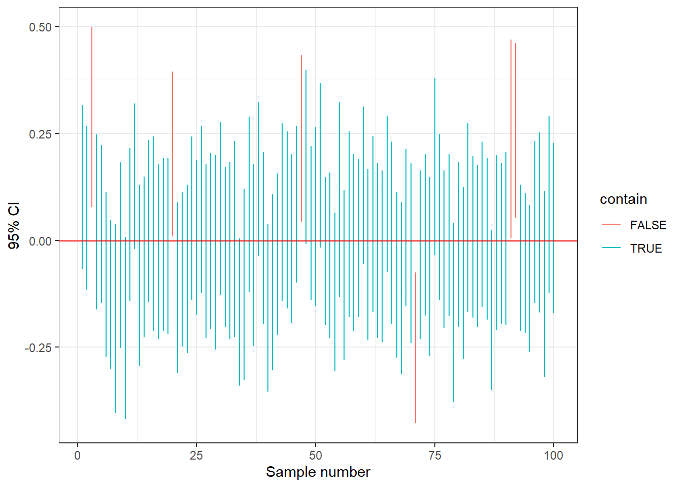

Exercise

Repeat the simulation study for a 90% confidence interval when the population parameter of interest is a proportion.

population <- rbinom(n = 100000, size = 1, prob = 0.2)
population_proportion <- mean(population)
population_proportion

(quant <- qnorm(1-0.10/2))

sample1 <- sample(population, 100)
phat <- mean(sample1)
ll <- phat - quant * sqrt(phat*(1-phat)/length(sample1))
ul <- phat + quant * sqrt(phat*(1-phat)/length(sample1))
c(ll, ul)

n <- 100  # sample size
M <- 1000 # number of samples
samples <- matrix(NA, nrow = M, ncol = n) # matrix with the samples
for(m in 1:M){
samples[m, ] <- sample(population, n)
}

ll <- apply(samples, 1,
FUN = function(samplem){
phat <- mean(samplem)
phat - quant * sqrt(phat*(1-phat)/length(samplem))
})

ul <- apply(samples, 1,
FUN = function(samplem){
phat <- mean(samplem)
phat + quant * sqrt(phat*(1-phat)/length(samplem))
})

mean(ll <= population_proportion & population_proportion <= ul)

library(ggplot2)
d <- data.frame(num = 1:M, ll = ll, ul = ul,
                contain = as.factor(ll <= population_proportion & population_proportion <= ul))
ggplot(data = d[1:100, ]) +
  geom_segment(aes(x = num, y = ll, xend = num, yend = ul, col = contain)) +
  geom_hline(yintercept = population_proportion, col = "red") +
  xlab("Sample number") + ylab("90% CI") + theme_bw()

4 Statistical inference

5 Confidence interval

6 Confidence interval for a proportion

6.1 Central Limit Theorem for a proportion

6.2 Confidence interval for a proportion

6.3 Example. Confidence interval for a proportion

6.4 Example. Confidence interval for a proportion

7 Confidence interval for a mean

7.1 Central Limit Theorem for the mean

7.2 Confidence interval for a mean

7.3 Confidence interval for a mean when \(\sigma\) is not known

7.4 Example. Confidence interval for a mean

7.5 Example. Confidence interval for a mean

8 Interpretation of a confidence interval