install.packages(c("sf", "terra", "geodata", "rnaturalearth", "spdep",
                   "dplyr", "SpatialEpi", "wbstats", "flexdashboard",
                   "ggplot2", "viridis", "RColorBrewer", "patchwork", "DT",
                   "leaflet", "mapview", "leafpop", "leafsync", "rasterVis"))

install.packages("INLA",
repos = c("https://inla.r-inla-download.org/R/stable", "https://cloud.r-project.org"), dep = TRUE)Spatial Data Science with R
Paula Moraga, Ph.D.
Assistant Professor of Statistics
King Abdullah University of Science
and Technology (KAUST), Saudi Arabia


Books
Geospatial Health Data: Modeling and Visualization (2019) http://www.paulamoraga.com/book-geospatial/

Manipulate and transform point, areal, raster data, create maps with R
Fit and interpret Bayesian spatial, spatio-temporal models with INLA, SPDE
Interactive visualizations, reproducible reports, dashboards and Shiny apps
Spatial Statistics for Data Science: Theory and Practice with R (2023) http://www.paulamoraga.com/book-spatial/
Spatial data: types, retrieval, manipulation and visualization. Statistical methods and models to analyze spatial data using R
Areal data: spatial neighborhood matrices, autocorrelation, models
Geostatistical data: interpolation, kriging, model-based geostatistics
Point patterns: intensity estimation, clustering, point process models
Reproducible examples in environment, ecology, epidemiology, crime, real estate

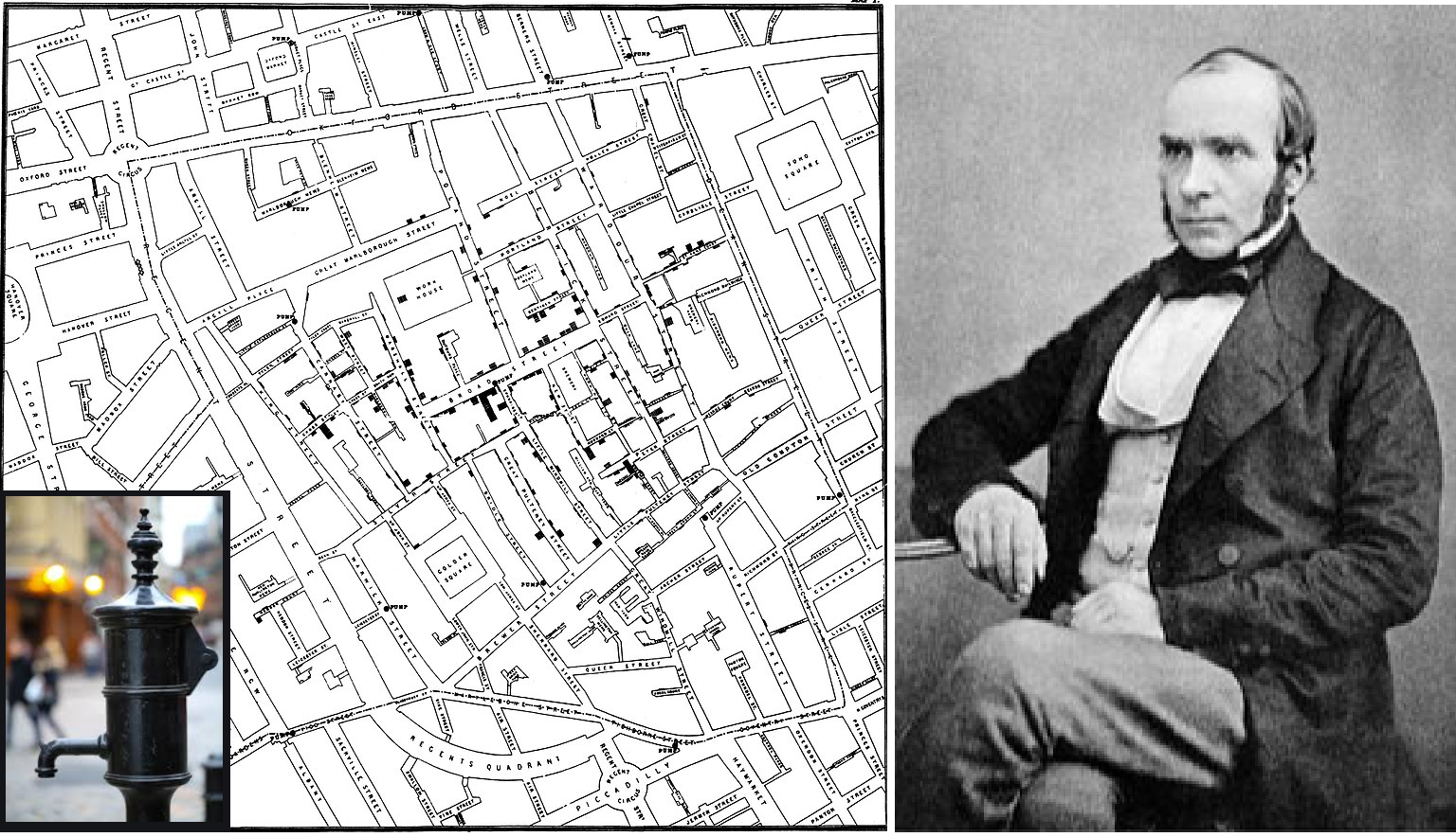
John Snow’s map of cholera, London, 1854
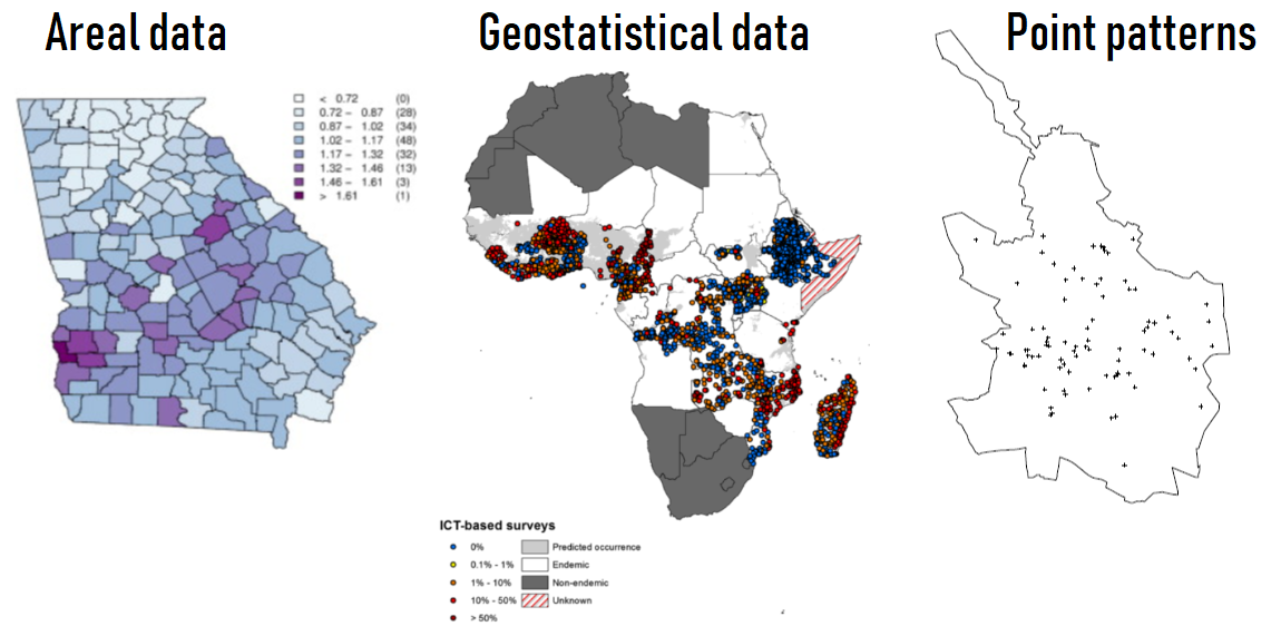
Types of spatial data
Moraga and Lawson, Computational Statistics & Data Analysis, 2012
Moraga et al., Parasites & Vectors, 2015
Moraga and Montes, Statistics in Medicine, 2011
Areal data
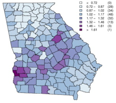
Model for disease relative risk \(\theta_i\) in areas
\[Y_i|\theta_i \sim Poisson(E_i \times \theta_i)\] \[\log(\theta_i) = \boldsymbol{z}_i \boldsymbol{\beta} + u_i + v_i\]
Fixed effects quantify the effects of the covariates on the disease risk
Random effects represent residual variation not explained by the covariates. \(u_i\) spatial effect to account for spatial dependence between relative risks. \(v_i\) unstructured effect to account for independent noise.
Moraga and Lawson, Computational Statistics & Data Analysis, 2012
Geostatistical data
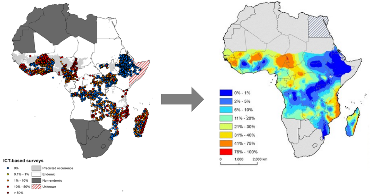
Geospatial modeling of lymphatic filariasis prevalence in sub-Saharan Africa
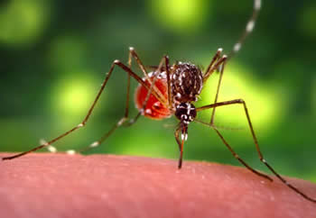
Lymphatic filariasis caused by microscopic worms and transmitted by mosquitoes
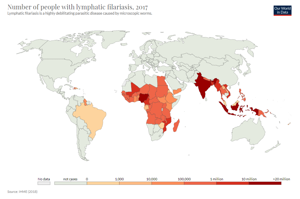
Main strategy against the disease is Mass Drug Administration. Resources are limited and need to decide which areas most in need

Geospatial modeling of lymphatic filariasis
\[Y_i|P(\boldsymbol{x}_i)\sim \mbox{Binomial} (n_i, P(\boldsymbol{x}_i)),\ \ \ \mbox{logit}(P(\boldsymbol{x}_i)) = \boldsymbol{z}_i \boldsymbol{\beta} + S(\boldsymbol{x}_i) + u_i\]
Covariates based on characteristics known to affect disease transmission (temperature, precipitation, vegetation, elevation, land cover, population, etc.). Random effects model residual variation not explained by covariates
Point patterns
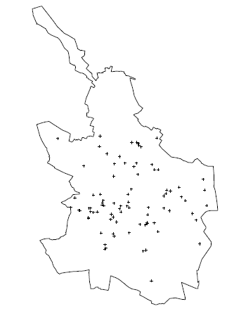
Assume point pattern \(\{s_i: i=1, \ldots, n\}\) has been generated as a realization of a point process \(Z = \{Z(s): s \in \mathbb{R}^2\}\)
A point process model can be used to estimate the intensity of events, identify patterns in the distribution of the observed locations, and learn about the correlation between the locations and spatial covariates
Types of spatial data
Moraga and Lawson, Computational Statistics & Data Analysis, 2012
Moraga et al., Parasites & Vectors, 2015
Moraga and Montes, Statistics in Medicine, 2011
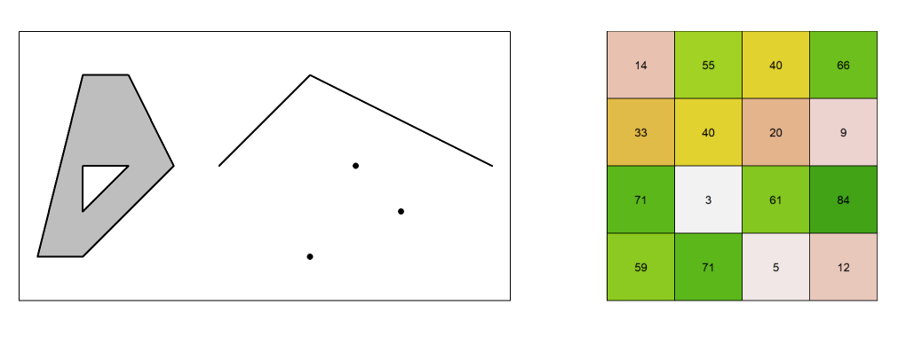
Spatial data in R
Spatial data can be represented using vector and raster data
Vector data displays points, lines and polygons, and associated information
Examples: locations of monitoring stations, road networks, municipalities
Raster data are regular grids with cells of equal size that are used to store values of spatially continuous phenomena
Examples: elevation, temperature, air pollution values
R packages: sf (vector data) and terra (raster and vector data)
sf to work with vector data
Vector data are often represented using a data format called shapefile.
library(sf)
pathshp <- system.file("shape/nc.shp", package = "sf")
map <- st_read(pathshp, quiet = TRUE)
plot(map[1])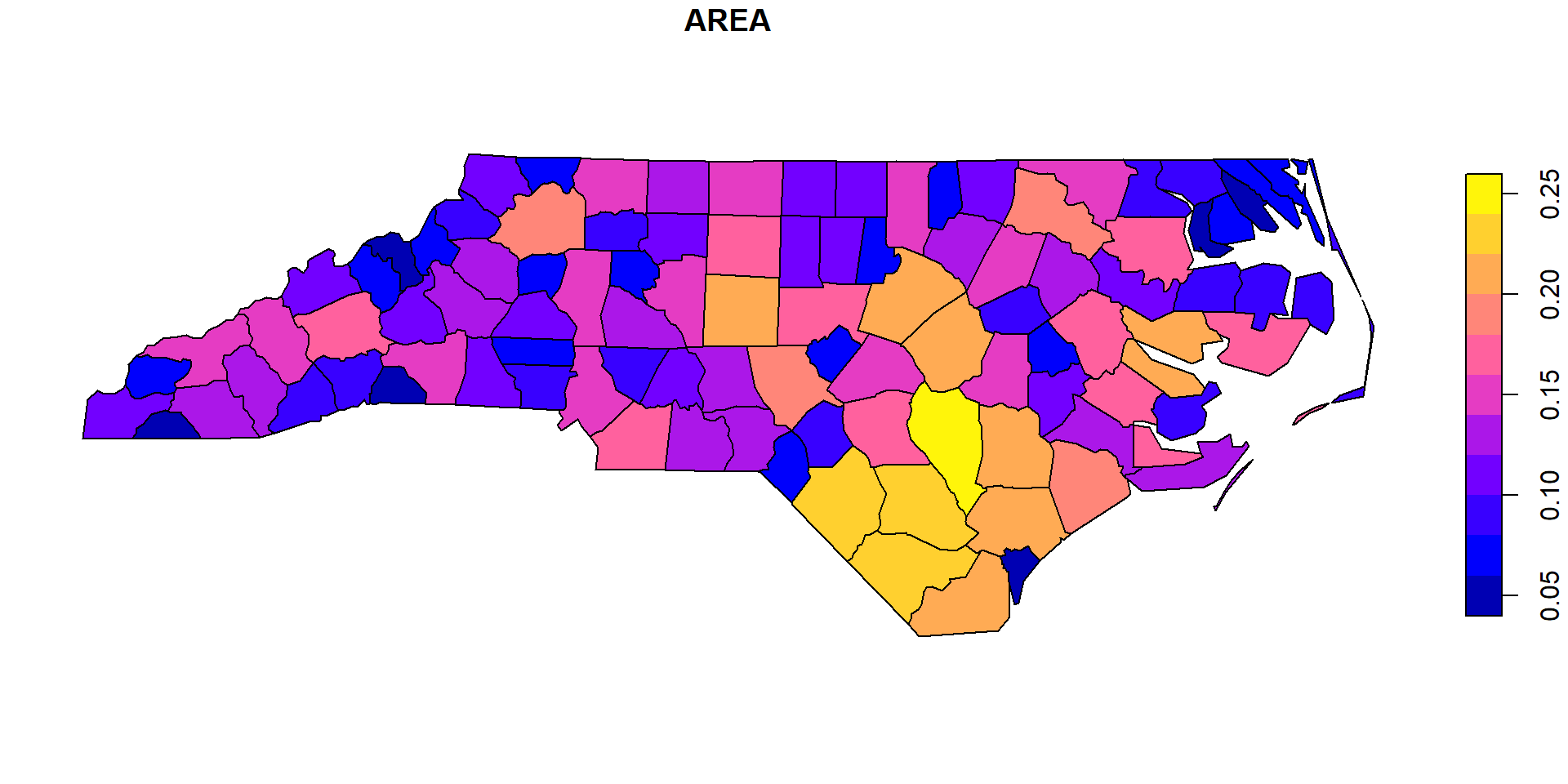
Shapefile to store vector data
A shapefile is a collection files.

terra to work with raster (and vector) data
Raster data often come in GeoTIFF format which has extension .tif.
library(terra)
pathraster <- system.file("ex/elev.tif", package = "terra")
r <- terra::rast(pathraster)
plot(r)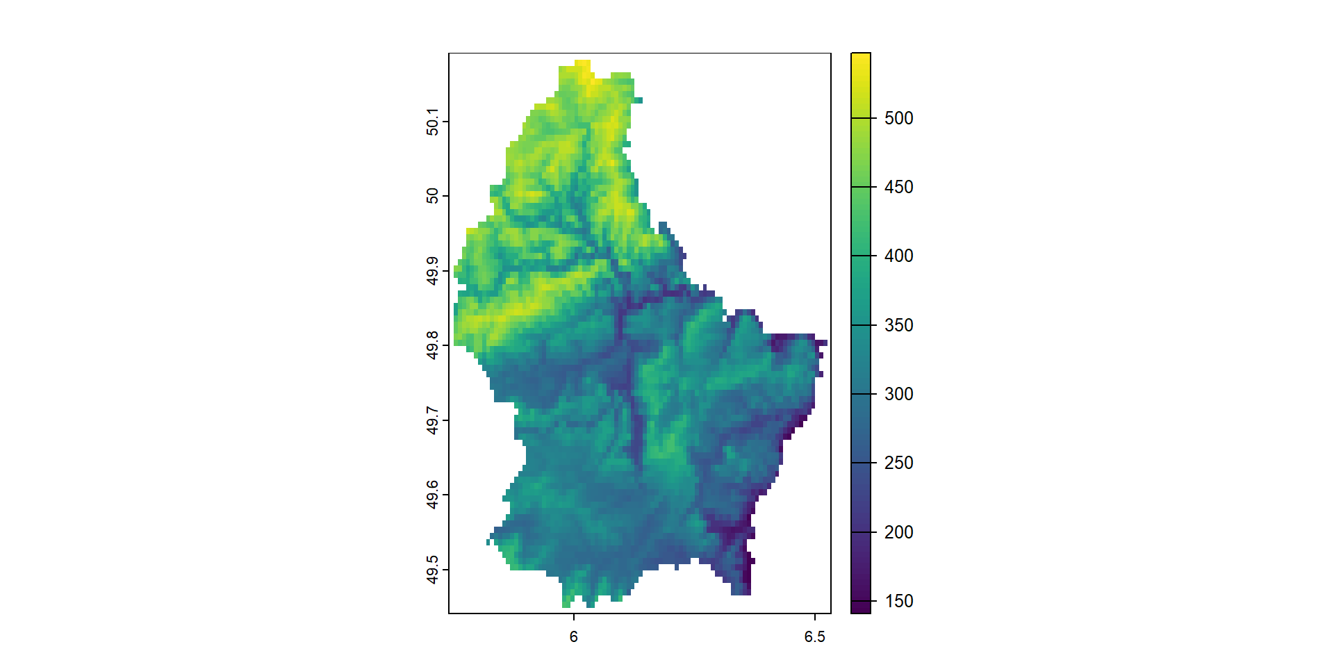
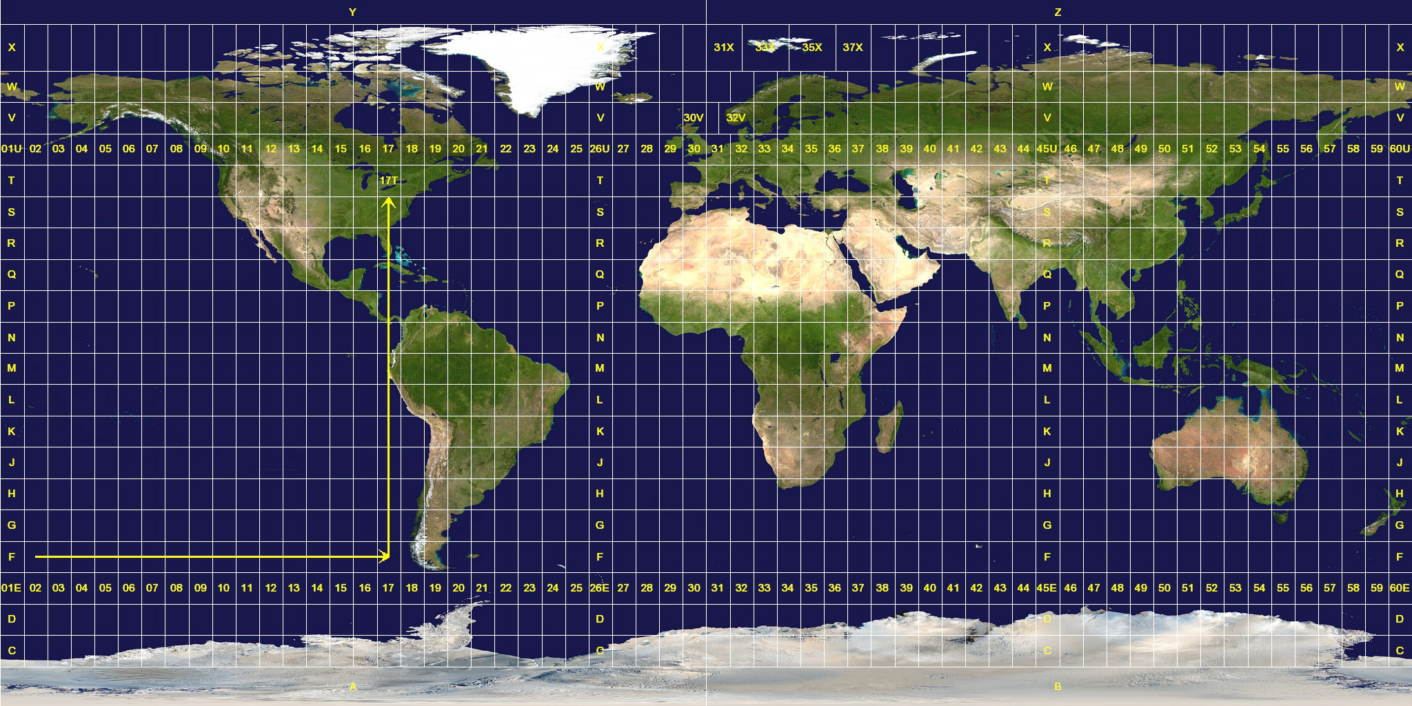
Coordinate Reference Systems (CRS)
unprojected or geographic: Latitude and Longitude for referencing location on the ellipsoid Earth
(decimal degrees (DD) or degrees, minutes, and seconds (DMS))projected: Easting and Northing for referencing location on 2-dimensional representation of Earth
Common projection: Universal Transverse Mercator (UTM)
Location is given by the zone number (60 zones), hemisphere (north or south), and Easting and Northing coordinates in the zone in meters

ggplot2
library(ggplot2)
library(viridis)
ggplot(d) + geom_sf(aes(fill = vble)) +
  scale_fill_viridis() + theme_bw()
tmap
library(tmap)
tmap_mode("plot") # Interactive with tmap_mode("view")
tm_shape(d) + tm_polygons("vble")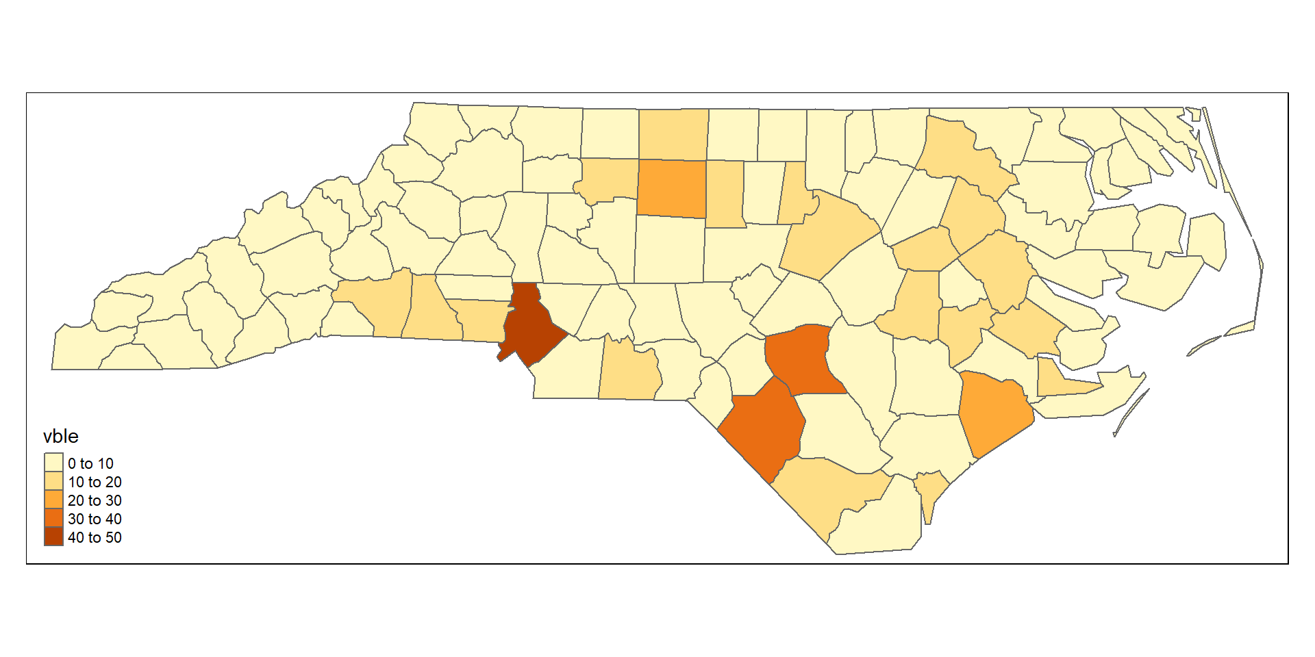
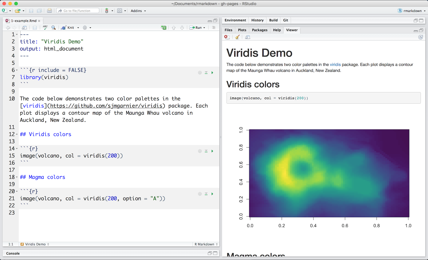
Reproducible documents with R Markdown
R Markdown can be used to turn our analysis into fully reproducible documents that can be shared with others. Output formats include HTML, PDF or Word. An R Markdown file is written with Markdown syntax with embedded R code, and can include narrative text, tables and visualizations
http://www.paulamoraga.com/book-geospatial/sec-rmarkdown.html
Interactive dashboards with flexdashboard
flexdashboard uses R Markdown to publish a group of related data visualizations as a dashboard
http://www.paulamoraga.com/book-geospatial/sec-flexdashboard.html
Shiny web applications
Shiny is a web application framework for R that enables to build interactive web applications
http://www.paulamoraga.com/book-geospatial/sec-shiny.html
SpatialEpiApp is a Shiny app for disease risk estimation, cluster detection, and interactive visualization
https://paulamoraga.shinyapps.io/spatialepiapp/
INLA
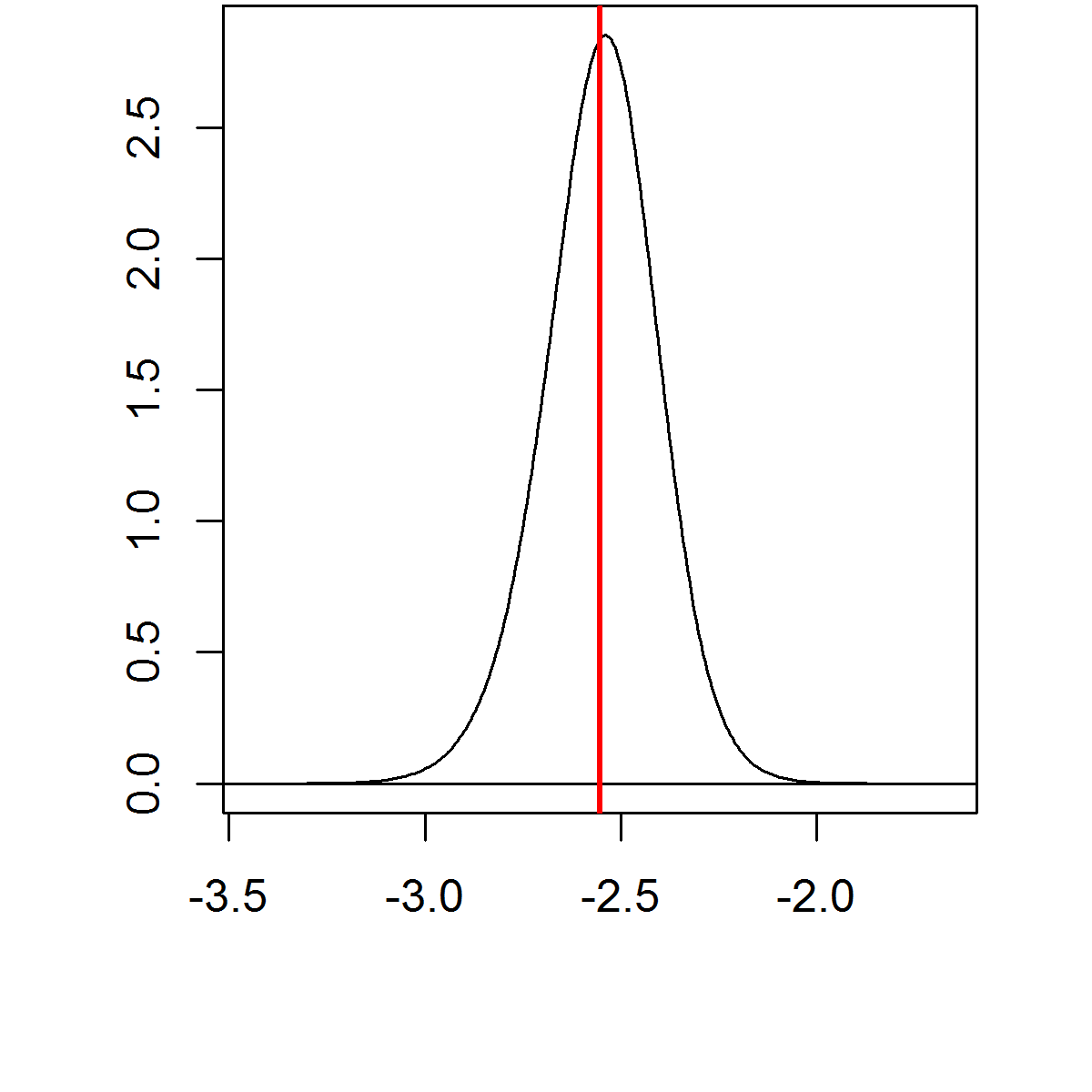
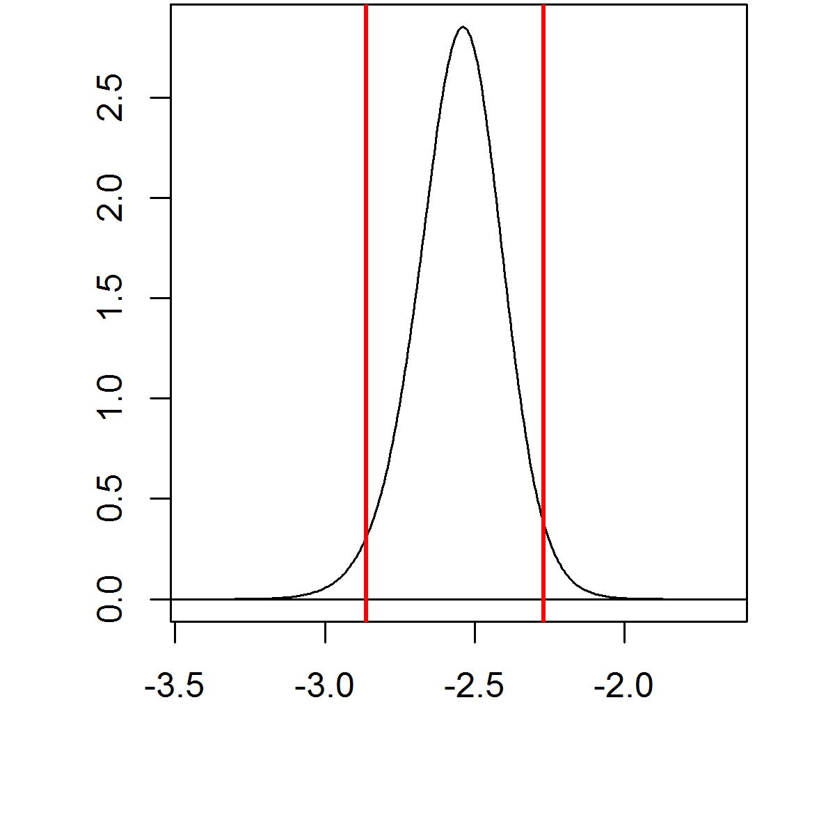
The approximated posterior distributions \(\tilde \pi (x_i|\boldsymbol{y})\) can be post-processed to compute quantities of interest like posterior expectations and quantiles
| Expectation | 95% C.I. |
|
|
Areal data
Standardized Mortality Ratio (SMR) is often used to estimate disease risk
\[ SMR_i = \frac{Y_i}{E_i} = \frac{\mbox{number observed cases in area } i}{\mbox{number expected cases in area } i}\]
\(SMR_i = 1\) same number observed as expected
\(SMR_i > 1\) more observed than exp. (high risk)
\(SMR_i < 1\) less observed than exp. (low risk)
Example
\(SMR_i = \frac{Y_i}{E_i} = \frac{200}{100} = 2 > 1\) \(\rightarrow\) area \(i\) high risk (observed \(>\) expected) \(SMR_i = \frac{Y_i}{E_i} = \frac{100}{200} = 0.5 < 1\) \(\rightarrow\) area \(i\) low risk (observed \(<\) expected)
Spatial neighborhood matrix
library(spdep)
nb <- poly2nb(map)

## [[1]]
## [1] 21 28 67
##
## [[2]]
## [1]  3  4 10 63 65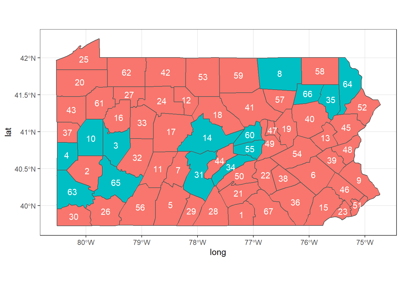
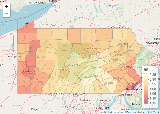
Visualization
library(leaflet)

pal <- colorNumeric(palette = "YlOrRd", domain = map$SIR)

leaflet(map) %>% addTiles() %>%
addPolygons(color = "grey", weight = 1, fillColor = ~ pal(SIR)) %>%
addLegend(pal = pal, values = ~SIR, title = "SIR")
Tutorial
Modeling areal data (lung cancer risk in Pennsylvania, USA)
https://www.paulamoraga.com/book-spatial/disease-risk-modeling.html
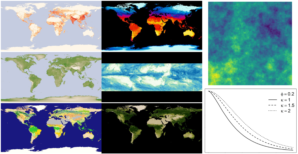
Geostatistical data
Geostatistical models
Models to predict prevalence at unsampled locations
\[Y_i|P(\boldsymbol{x}_i)\sim \mbox{Binomial} (n_i, P(\boldsymbol{x}_i))\] \[\mbox{logit}(P(\boldsymbol{x}_i)) = \boldsymbol{z}_i \boldsymbol{\beta} + S(\boldsymbol{x}_i) + u_i\]
\(Y_i\) number people positive, \(n_i\) number people tested, \(P(\boldsymbol{x}_i)\) prevalence at \(\boldsymbol{x}_i\)
Covariates based on characteristics known to affect disease transmission (temperature, precipitation, vegetation, elevation, land cover, population density, etc.)
Random effects model residual variation not explained by covariates
Inference using INLA and SPDE
Integrated nested Laplace approximations (INLA) is a computational approach to perform approximate Bayesian inference in latent Gaussian models
In the Stochastic partial differential equation (SPDE) approach, the continuously indexed Gaussian random field \(S\) is represented as a discretely indexed Gaussian Markov random field (GMRF) by means of a finite basis function defined on a triangulation of the study region
\[S(\boldsymbol{x}) = \sum_{g=1}^G \psi_g(\boldsymbol{x}) S_g\]
\(\psi_g(\cdot)\) piecewise polynomial basis functions on each triangle
\(\{S_g \}\) zero-mean Gaussian distributed
\(G\) number of vertices in triangulation
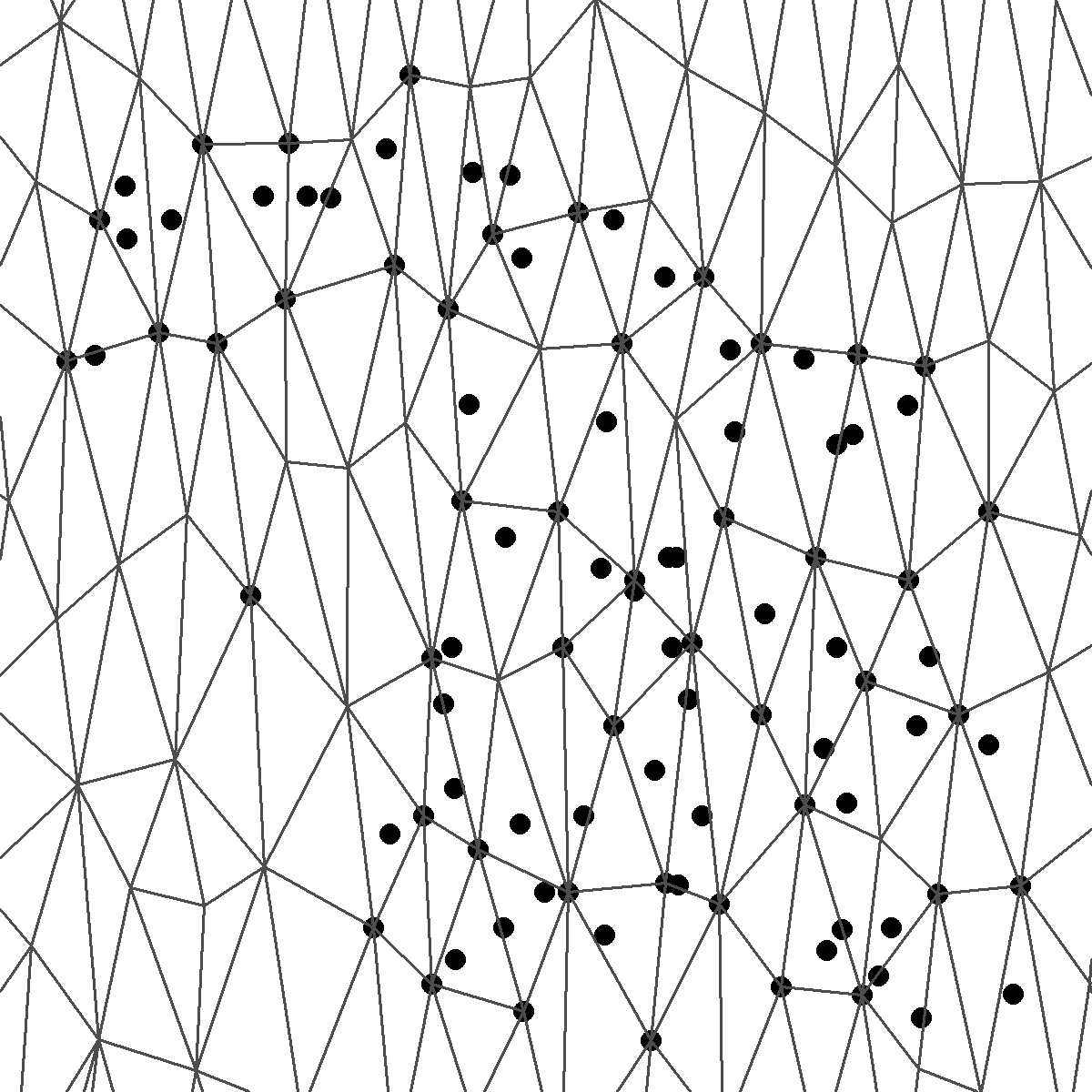
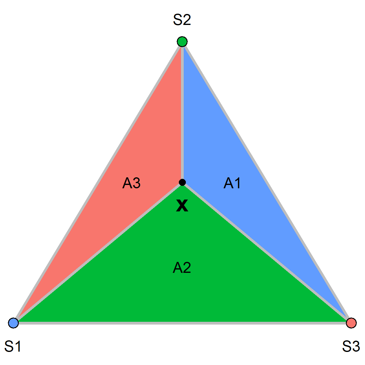
Projection matrix
\(S(\boldsymbol{x})\) weighted average of the GMRF values at the vertices of the triangle containing the point. Weights = barycentric coordinates
\[S(\boldsymbol{x}) \approx \frac{T_{1}}{T}S_1 + \frac{T_{2}}{T}S_2 + \frac{T_{3}}{T}S_3\]
\(T_1, T_2, T_3\) areas subtriangles formed by \(\boldsymbol{x}\) and vertices. \(T\) area whole triangle
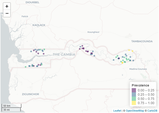
Tutorial
Modeling geostatistical data (malaria prevalence in The Gambia)
https://www.paulamoraga.com/book-geospatial/sec-geostatisticaldataexamplespatial.html
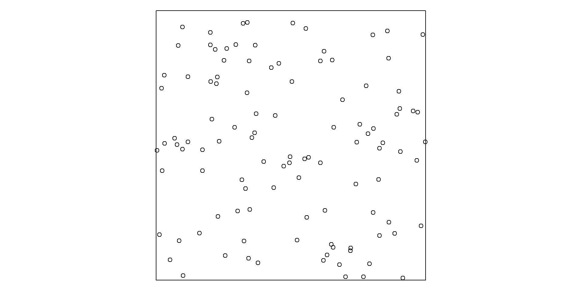
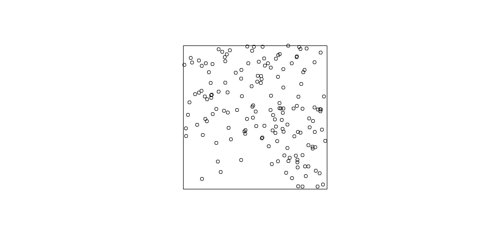
Point patterns
Assume point pattern \(\{s_i: i=1, \ldots, n\}\) has been generated as a realization of a point process \(Z = \{Z(s): s \in \mathbb{R}^2\}\)
A point process model can be used to estimate the intensity of events, identify patterns in the distribution of the observed locations, and learn about the correlation between the locations and spatial covariates
Intensity of the process
Intensity of the process: mean number of events per unit area at location \(s\) \[\lambda(s) = lim_{|ds|\rightarrow 0} \frac{E[N(ds)]}{|ds|}\]
library(spatstat)
plot(X)
den <- density(x = X, sigma = 10)
plot(den, main = "Intensity")
contour(den, add = TRUE)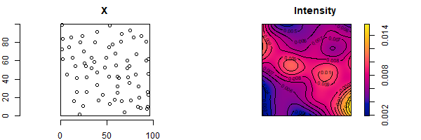
Complete Spatial Randomness
Point processes are stochastic models that describe the locations of events of interest and possibly some additional information such as marks that inform about different types of events (e.g., cases and controls)
Point processes provide models for point patterns, with complete spatial randomness (CSR) being the simplest theoretical model
CSR helps differentiate between regular and clustered patterns
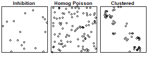
Homogeneous Poisson process (CSR)
Simple model that assumes events are equally likely to occur at any location within the study area, independent of the locations of other events
- the number of events in any region \(A\) follows a Poisson distribution with mean \(\lambda |A|\), where \(\lambda\) is a constant value denoting the intensity and \(|A|\) is the area of \(A\)
- given that there are \(n\) events inside \(A\), the locations of these events are independent and uniformly distributed in \(A\)
Inhomogeneous Poisson process
In homogeneous Poisson processes, the intensity is constant (\(\lambda(s)= \lambda,\ \ \forall s\)), whereas in inhomogeneous Poisson processes, the intensity varies in space.
- the number of events in any region \(A\) follows a Poisson distribution with mean \(\mu(A) = \int_A \lambda(s)ds\)
- given that there are \(n\) events inside \(A\), the locations of these events are independent with probability density function proportional to the intensity \(\lambda(\cdot)\)
Fitting a log-Gaussian Cox process model
Assume point pattern \(\{s_i: i=1, \ldots, n\}\) has been generated as a realization of a LGCP with intensity \(\Lambda(s)= exp(\eta(s))\)
A LGCP can be fitted by discretizing the study region into a grid with \(n_1 \times n_2\) cells \(\{s_{ij}: i=1,\ldots,n_1, j=1,\ldots,n_2\}\). \(|s_{ij}|\) area of cell \(s_{ij}\)
Mean number of events in cell \(s_{ij}\):
\(\Lambda_{ij}=\int_{s_{ij}} exp(\eta(s))ds \approx |s_{ij}| exp(\eta_{ij})\)
\(y_{ij}|\eta_{ij} \sim Poisson(|s_{ij}| exp(\eta_{ij}))\)
\(\eta_{ij} = \beta_0 + \beta_1 \times cov(s_{ij}) + f_s(s_{ij}) + f_u(s_{ij})\)
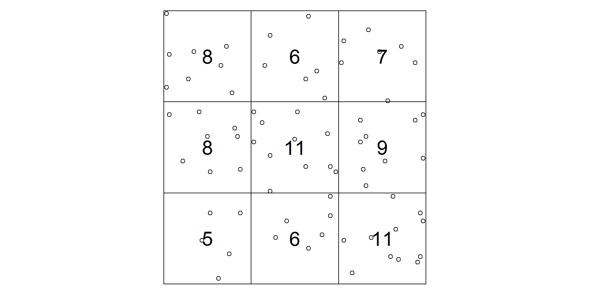
- \(y_{ij}\) observed number of locations in grid cell \(s_{ij}\)
- \(\beta_0\) intercept, \(cov(s_{ij})\) covariate at \(s_{ij}\), \(\beta_1\) coefficient of \(cov(s_{ij})\)
- \(f_s()\) spatially structured random effect (CAR model on a regular lattice)
- \(f_u()\) unstructured random effect
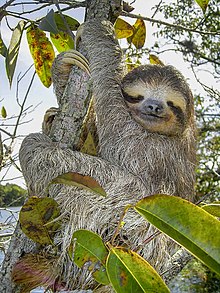
Tutorial
Modeling point patterns (sloths occurrence in Costa Rica)
http://www.paulamoraga.com/tutorial-point-patterns
spocc package: https://docs.ropensci.org/spocc/
R Markdown
R Markdown can be used to turn our analysis into fully reproducible documents that can be shared with others. Output formats include HTML, PDF or Word. An R Markdown file is written with Markdown syntax with embedded R code, and can include narrative text, tables and visualizations
http://www.paulamoraga.com/book-geospatial/sec-rmarkdown.html
R Markdown
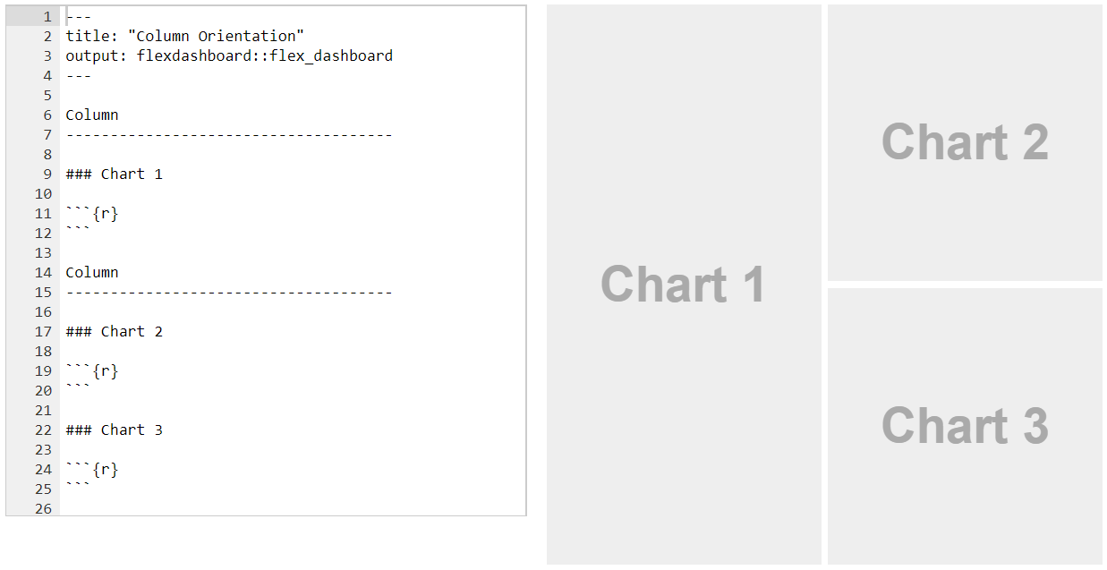
Dashboards with flexdashboard
The R package flexdashboard uses R Markdown to publish a group of related data visualizations as a dashboard
http://www.paulamoraga.com/book-geospatial/sec-flexdashboard.html
Layout
Dashboards with flexdashboard
Tutorial
Interactive dashboards with flexdashboard to communicate results
https://www.paulamoraga.com/book-geospatial/sec-flexdashboard
Example (lung cancer risk in Pennsylvania, USA)
http://www.paulamoraga.com/tutorial-flexdashboard-example
SpatialEpiApp
SpatialEpiApp is a Shiny app for disease risk estimation, cluster detection, and interactive visualization
- Risk estimates by fitting Bayesian models with INLA
- Detection of clusters by using the scan statistics in SaTScan
devtools::install_github("Paula-Moraga/SpatialEpiApp")
library(SpatialEpiApp); run_app()Inputs
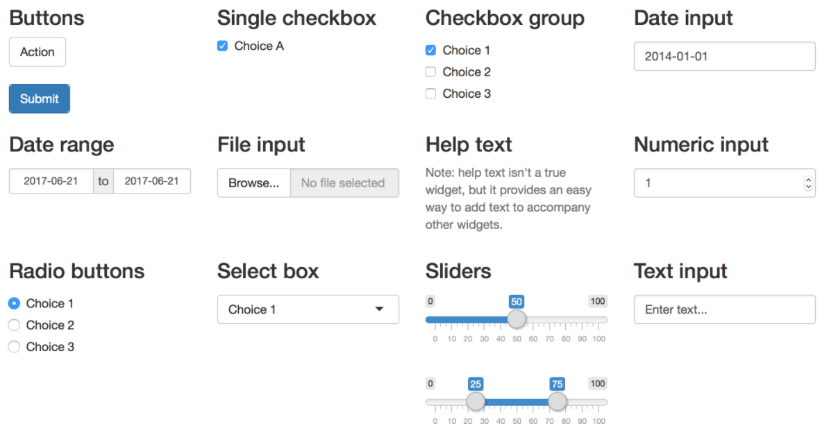
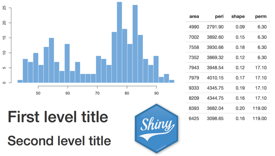
Outputs
Plots, tables, texts, images
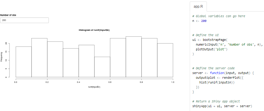
Inputs, outputs and reactivity
https://shiny.posit.co/r/gallery/start-simple/single-file-shiny-app/
Interactive dashboards with
flexdashboard and Shiny
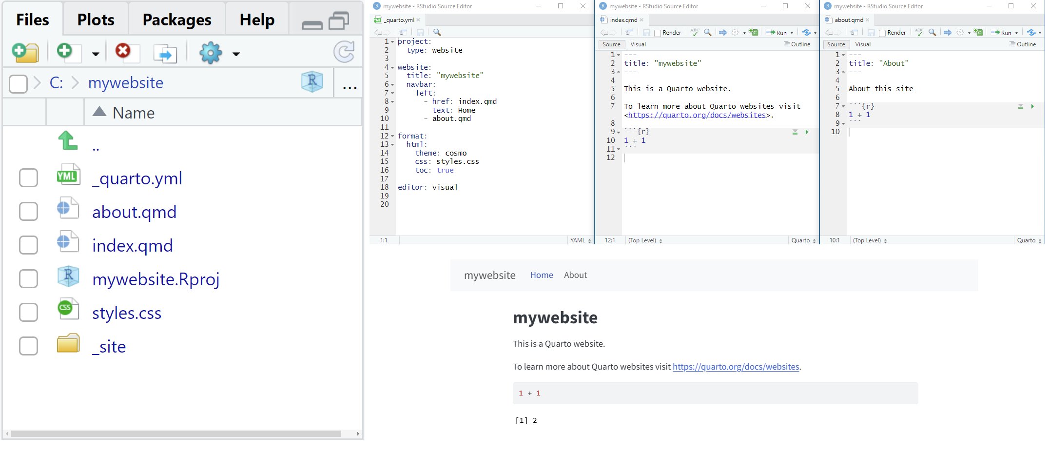
Quarto websites
File > New Project > New Directory > Quarto Website
Click Render
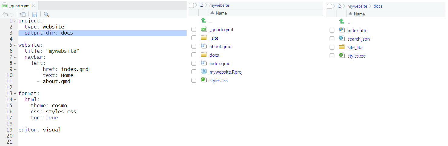
Render website to the docs directory
Add out-dir: docs to _quarto.yml to render website to the docs directory
GitHub Pages
Configure GitHub repo to publish from the docs directory
In GitHub, go to Settings, Pages, select master, select /docs, and click on Save
Your site is live at http://www.paulamoraga.com/mywebsite/

References
Ribeiro Amaral, A., et al. (2022). Spatio-temporal modeling of infectious diseases by integrating compartment and point process models. SERRA, 37, 1519-1533
Moraga, P. and Baker, L. (2022). rspatialdata: a collection of data sources and tutorials on downloading and visualising spatial data using R. F1000Research, 11:77
Moraga, P., et al. (2019). epiflows: an R package for risk assessment of travel-related spread of disease. F1000Research, 7:1374
Moraga, P. (2018). Small Area Disease Risk Estimation and Visualization Using R. The R Journal, 10(1):495-506
Moraga, P. (2017). SpatialEpiApp: A Shiny Web Application for the analysis of Spatial and Spatio-Temporal Disease Data. Spatial and Spatio-temporal Epidemiology, 23:47-57
Moraga, P., et al. (2017). A geostatistical model for combined analysis of point-level and area-level data using INLA and SPDE. Spatial Statistics, 21:27-41
Moraga, P. and Kulldorff, M. (2016). Detection of spatial variations in temporal trends with a quadratic function. Statistical Methods for Medical Research, 25(4):1422-1437
Hagan, J. E., Moraga, P., et al. (2016). Spatio-temporal determinants of urban leptospirosis transmission: Four-year prospective cohort study of slum residents in Brazil. PLOS Neglected Tropical Diseases, 10(1): e0004275
Moraga, P., et al. (2015). Modelling the distribution and transmission intensity of lymphatic filariasis in sub-Saharan Africa prior to scaling up interventions: integrated use of geostatistical and mathematical modelling. Parasites & Vectors, 8:560