15 Model-based geostatistics
Model-based geostatistics can be used to analyze spatial data related to an underlying spatially continuous phenomenon that have been collected at a finite set of locations. Model-based geostatistics employs statistical models to capture the spatial correlation structure in the data, enabling rigorous statistical inference, and facilitating the production of spatial predictions along with uncertainty measures of the phenomenon of interest (Diggle, Tawn, and Moyeed 1998).
Assuming Gaussian data observed at a set of \(n\) locations, \(\{Y_1, \ldots, Y_n\}\), we can consider the following model to obtain predictions at unsampled locations:
\[Y_i | S(\boldsymbol{s}_i) \sim N(\mu + S(\boldsymbol{s}_i), \tau^2), i = 1,\ldots,n.\]
Here, \(\mu\) is a constant mean effect, and \(S(\cdot)\) is a zero-mean spatial Gaussian field. This model can be extended to situations in which the stochastic variation in the data is not Gaussian, as well as to include covariates and other random effects to account for other types of variability.
Inference in model-based geostatistics can be performed using the INLA and the stochastic partial differential equation (SPDE) approaches which provide a computationally efficient alternative to MCMC methods (Lindgren and Rue 2015). Briefly, this involves solving a SPDE on a discrete mesh of points and interpolating to obtain a continuous solution across the spatial domain (Krainski et al. 2019) which is calculated using INLA (Rue, Martino, and Chopin 2009).
Model-based geostatistics using INLA and SPDE has been employed for spatial prediction in a wide range of applications including air pollution in Italy (Cameletti et al. 2013), leptospirosis in Brazil (Hagan et al. 2016), and malaria in Mozambique (Moraga et al. 2021). Model-based geostatistics also provides a flexible approach to combine multiple data available at different spatial resolutions to get better predictions than the ones obtained using just one type of data (Zhong and Moraga 2023). For example, Moraga et al. (2017) demonstrate how to integrate air pollution measures obtained at a collection of monitoring stations, and aggregated at cells of a regular grid derived from satellites to obtain predictions at a continuous surface and improve decision-making. Moreover, model-based geostatistics can also account for preferential sampling that may occur when the spatial phenomenon of interest and the sampling locations exhibit stochastic dependence (Diggle, Menezes, and Su 2010). Specifically, spatially misaligned data can be combined by assuming a common spatial random field underlying all observations. In the integration of data, preferential sampling can be taken into account by assuming a shared spatial random process by both the measured observations and the intensity of the point process that originates the locations, with a parameter controlling the degree of preferential sampling (Zhong, Ribeiro Amaral, and Moraga 2023; Ribeiro Amaral et al. 2023).
In this chapter, we introduce the SPDE approach, and show how to specify, fit, and interpret a geostatistical model to predict air pollution in the USA using INLA and SPDE. Additional examples on how to implement the INLA and SPDE approaches to fit geostatistical models are provided in Krainski et al. (2019) and Moraga (2019). Specifically, Moraga (2019) demonstrates how to fit both spatial and spatio-temporal models to predict malaria prevalence in The Gambia, precipitation in Brazil, and air pollution in Spain.
15.1 The SPDE approach
The stochastic partial differential equation (SPDE) approach implemented in the R-INLA package provides a flexible and computationally efficient way to model geostatistical data and make predictions at unsampled locations (Lindgren and Rue 2015). We assume that underlying the observed data, there is a spatially continuous variable that can be modeled using a Gaussian random field (GRF) with Matérn covariance function which is defined as
\[\mbox{Cov}(x(\boldsymbol{s}_i), x(\boldsymbol{s}_j))=\frac{\sigma^2}{2^{\nu-1}\Gamma(\nu)}(\kappa ||\boldsymbol{s}_i - \boldsymbol{s}_j ||)^\nu K_\nu(\kappa ||\boldsymbol{s}_i - \boldsymbol{s}_j ||).\]
Here, \(\sigma^2\) denotes the marginal variance of the spatial field. \(K_\nu(\cdot)\) refers to the modified Bessel function of second kind and order \(\nu>0\). The integer value of \(\nu\) determines the smoothness of the field and is typically fixed since it is difficult to estimate in applications. \(\kappa >0\) is related to the range \(\rho\), which represents the distance at which the correlation between two points becomes approximately 0. Specifically, \(\rho = \sqrt{8\nu}/\kappa,\) and at this distance the spatial correlation is close to 0.1 (Cameletti et al. 2013).
As shown in Whittle (1963), a GRF with a Matérn covariance matrix can be represented as a solution of the following continuous domain SPDE:
\[(\kappa^2 - \Delta)^{\alpha/2}(\tau x(\boldsymbol{s})) = \mathcal{W}(\boldsymbol{s}).\]
Here, \(x(\boldsymbol{s})\) represents a GRF, and \(\mathcal{W}(\boldsymbol{s})\) is a Gaussian spatial white noise process. The parameter \(\alpha\) controls the smoothness exhibited by the GRF, \(\tau\) controls its variance, and \(\kappa >0\) is a scale parameter. The Laplacian \(\Delta\) is defined as \(\sum_{i=1}^d \frac{\partial^2}{\partial x^2_i}\), where \(d\) is the dimension of the spatial domain.
The parameters of the Matérn covariance function and the SPDE are related as follows. The smoothness parameter \(\nu\) of the Matérn covariance function is expressed as \(\nu = \alpha - \frac{d}{2}\), and the marginal variance \(\sigma^2\) is related to the SPDE through
\[\sigma^2 = \frac{\Gamma(\nu)}{\Gamma(\alpha)(4\pi)^{d/2}\kappa^{2\nu}\tau^2}.\]
In the case where \(d=2\) and \(\nu=1/2\), which corresponds to the exponential covariance function, the parameter \(\alpha = \nu + d/2 =1/2+1=3/2\). In the R-INLA package, the default value is \(\alpha = 2\), although options within the range \(0\leq \alpha < 2\) are also available.
The Finite Element method can be used to find an approximate solution to the SPDE. This method involves dividing the spatial domain into a set of non-intersecting triangles, creating a triangulated mesh with \(n\) nodes and \(n\) basis functions. The basis functions, denoted as \(\psi_k(\cdot)\), are piecewise linear functions on each triangle. They take the value of 1 at vertex \(k\), and 0 at all other vertices.
Then, the continuously indexed Gaussian field \(x\) is represented as a discretely indexed Gaussian Markov random field (GMRF) by a sum of basis functions defined on the triangulated mesh
\[x(\boldsymbol{s})=\sum_{k=1}^n \psi_k(\boldsymbol{s}) x_k,\] where \(n\) is the number of vertices of the triangulation, \(\psi_k(\cdot)\) represents the piecewise linear basis functions, and \(\{x_k\}\) denote zero-mean Gaussian distributed weights.
The joint distribution of the weight vector is assigned a Gaussian distribution represented as \(\boldsymbol{x}=({x}_1,\ldots,{x}_n) \sim N(\boldsymbol{0}, \boldsymbol{Q}^{-1}(\tau, \kappa))\). This distribution approximates the solution \(x(\boldsymbol{s})\) of the SPDE at the mesh nodes. The basis functions transform the approximation \(x(\boldsymbol{s})\) from the mesh nodes to the other spatial locations of interest.
Projection matrix
The SPDE approach can be implemented with R-INLA by creating a projection matrix \(A\) that projects the GRF from the observations to the vertices of the triangulated mesh. The projection matrix \(A\) has a number of rows equal to the number of observations, and a number of columns equal to the number of vertices of the mesh. Each row \(i\) of \(A\) corresponds to an observation at location \(\boldsymbol{s}_i\), and may have up to three non-zero values in the columns that correspond to the vertices of the triangle containing the location. If \(\boldsymbol{s}_i\) lies within the triangle, these values are equal to the barycentric coordinates. In other words, they are proportional to the areas of each of the three subtriangles formed by the location \(\boldsymbol{s}_i\) and the triangle’s vertices, and they sum to 1. If \(\boldsymbol{s}_i\) coincides with a vertex of the triangle, row \(i\) has just one non-zero value equal to 1 in the column that corresponds to that vertex.
For example, the projection matrix below has \(n\) rows as the number of observations, and \(G\) columns as the number of vertices of the triangulated mesh. The first row of the matrix corresponds to an observation located at the vertex in the third position. The second and last rows correspond to observations located within triangles.
\[ A = \begin{bmatrix} A_{11} & A_{12} & A_{13} & \dots & A_{1G} \\ A_{21} & A_{22} & A_{23} & \dots & A_{2G} \\ \vdots & \vdots & \vdots & \ddots & \vdots \\ A_{n1} & A_{n2} & A_{n3} & \dots & A_{nG} \end{bmatrix} = \begin{bmatrix} 0 & 0 & 1 & \dots & 0 \\ A_{21} & A_{22} & 0 & \dots & A_{2G} \\ \vdots & \vdots & \vdots & \ddots & \vdots \\ A_{n1} & A_{n2} & A_{n3} & \dots & 0 \end{bmatrix} \]
Figure 15.1 shows a location \(\boldsymbol{s}\) within one of the triangles of a triangulated mesh. The value of the process \(Z(\cdot)\) at \(\boldsymbol{s}\) is determined through a weighted average of the process values at the triangle’s vertices \((Z_1, Z_2, Z_3)\). These weights are calculated by dividing the areas of the subtriangles \((T_1, T_2, T_3)\) by the area of the larger triangle that contains \(\boldsymbol{s}\) (\(T\)):
\[Z(\boldsymbol{s}) \approx \frac{T_1}{T} Z_1 + \frac{T_2}{T} Z_2 + \frac{T_3}{T} Z_3.\]
Thus, the value \(Z(\boldsymbol{s})\) at a location within a mesh triangle can be obtained by projecting the plane formed by the triangle vertices weights at location \(\boldsymbol{s}\).
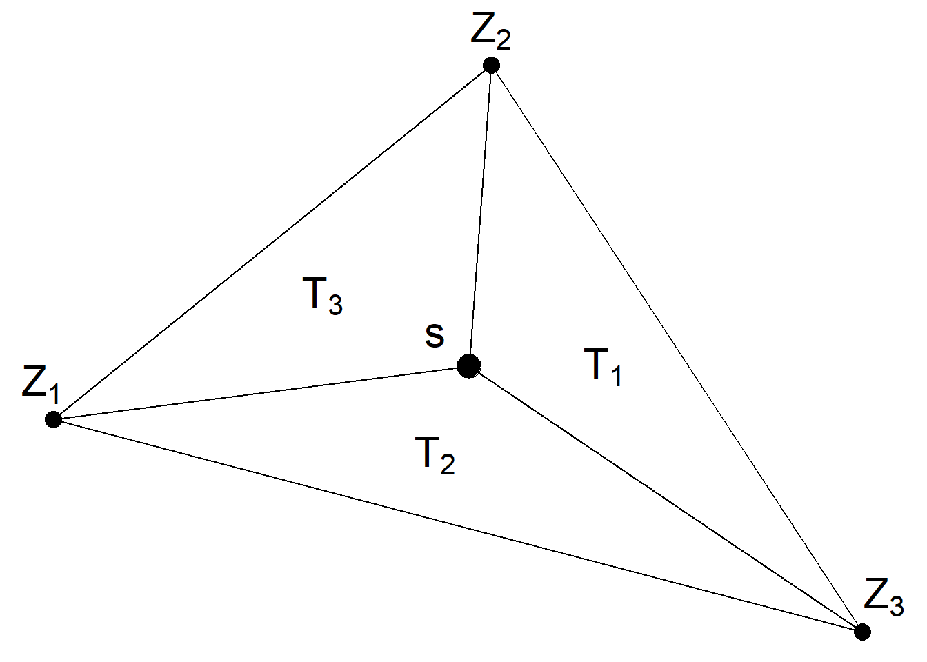
FIGURE 15.1: Triangle of a triangulated mesh.
15.2 Air pollution prediction
In this section, we show how to fit a geostatistical model to predict fine particulate matter PM2.5 in the USA using the INLA and SPDE approaches.
15.2.1 Observed PM2.5 values in the USA
Annual averages of PM2.5 concentration levels recorded at 1429 monitoring stations from the United States Environmental Protection Agency in 2022 are in the PM25USA2022.csv file that can be downloaded from
this website.
We use the read.csv() function to read the data which contains the longitude and latitude values of the monitoring stations, and the recorded PM2.5 values in micrograms per cubic meter.
Then, we use the st_as_sf() function to transform the data.frame obtained to a sf object with geographic CRS given by EPSG code 4326.
library(sf)
f <- file.path("https://www.paulamoraga.com/book-spatial/",
               "data/PM25USA2022.csv")
d <- read.csv(f)
d <- st_as_sf(d, coords = c("longitude", "latitude"))
st_crs(d) <- "EPSG:4326"
We then obtain the map of the USA with the ne_countries() function of rnaturalearth. We use st_crop() to remove Alaska and other areas that are outside the region comprised by longitude values (–130, 60) and latitude values (18, 72).
library(rnaturalearth)
map <- ne_countries(type = "countries",
                    country = "United States of America",
                    scale = "medium", returnclass = "sf")
map <- st_crop(map, xmin = -130, xmax = -60, ymin = 18, ymax = 72)
We then keep the 1366 monitoring stations locations that are within the map by using the st_filter() function.
[1] 1366Figure 15.2 shows a map with the PM2.5 observed values.
15.2.2 Prediction data
Here, we construct a matrix coop with the locations where the air pollution levels will be predicted.
First, we create a raster grid with 100 \(\times\) 100 cells covering the map using the rast() function of terra. Then, we obtain the coordinates of the cells with the xyfromCell() function of terra.
library(sf)
library(terra)

# raster grid covering map
grid <- terra::rast(map, nrows = 100, ncols = 100)
# coordinates of all cells
xy <- terra::xyFromCell(grid, 1:ncell(grid))
Then, we use the st_as_sf() function to create a sf object with the coordinates of the prediction locations by specifying the coordinates as a data frame, the name of the coordinates, and the CRS.
We obtain the indices of the point coordinates that are within the map with st_intersects() setting sparse = FALSE. We will later use these indices to identify the prediction locations. We also obtain the point coordinates that are within the map with sf_filter().
Figure 15.2 shows the prediction locations.
# transform points to a sf object
dp <- st_as_sf(as.data.frame(xy), coords = c("x", "y"),
                 crs = st_crs(map))

# indices points within the map
indicespointswithin <- which(st_intersects(dp, map,
                                           sparse = FALSE))

# points within the map
dp <- st_filter(dp, map)

# plot
ggplot() + geom_sf(data = map) +
  geom_sf(data = dp)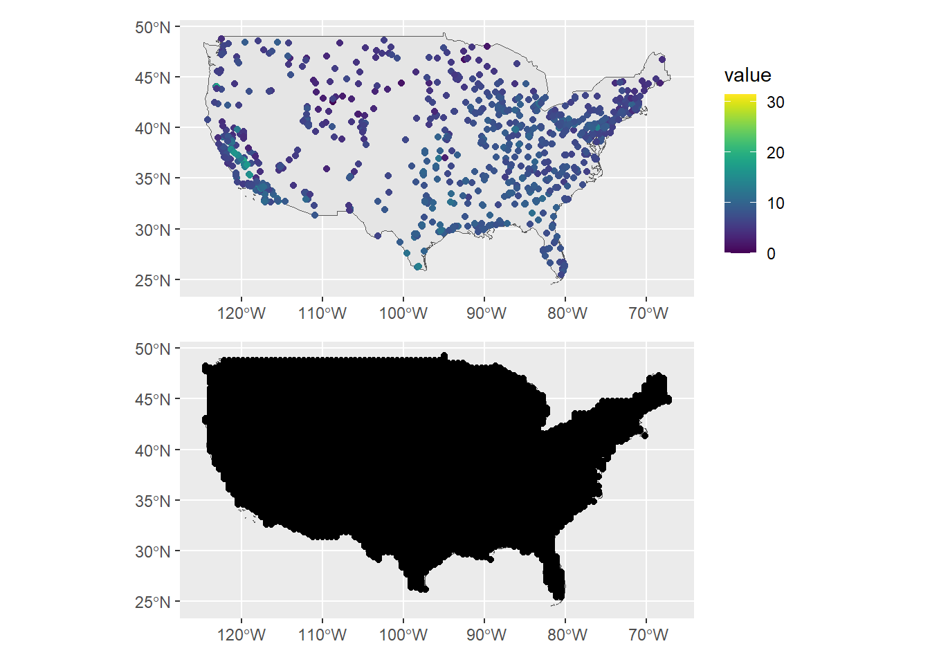
FIGURE 15.2: Map with the PM2.5 observed values (top) and prediction locations (bottom).
15.2.3 Covariates
In our model, we use average temperature and precipitation as covariates.
Monthly values of these variables globally can be obtained with the worldclim_global() function of geodata.
library(geodata)
covtemp <- worldclim_global(var = "tavg", res = 10,
                            path = tempdir())
covprec <- worldclim_global(var = "prec", res = 10,
                            path = tempdir())
After downloading the data, we compute the averages over months and extract the values at the observation and prediction locations with the extract() function of terra.
# Extract at observed locations
d$covtemp <- extract(mean(covtemp), st_coordinates(d))[, 1]
d$covprec <- extract(mean(covprec), st_coordinates(d))[, 1]
# Extract at prediction locations
dp$covtemp <- extract(mean(covtemp), st_coordinates(dp))[, 1]
dp$covprec <- extract(mean(covprec), st_coordinates(dp))[, 1]
Figure 15.3 shows maps of the temperature and precipitation covariates at the observation locations created with the ggplot2 and patchwork packages.
library("patchwork")
p1 <- ggplot() + geom_sf(data = map) +
  geom_sf(data = d, aes(col = covtemp)) +
  scale_color_viridis()
p2 <- ggplot() + geom_sf(data = map) +
  geom_sf(data = d, aes(col = covprec)) +
  scale_color_viridis()
p1 / p2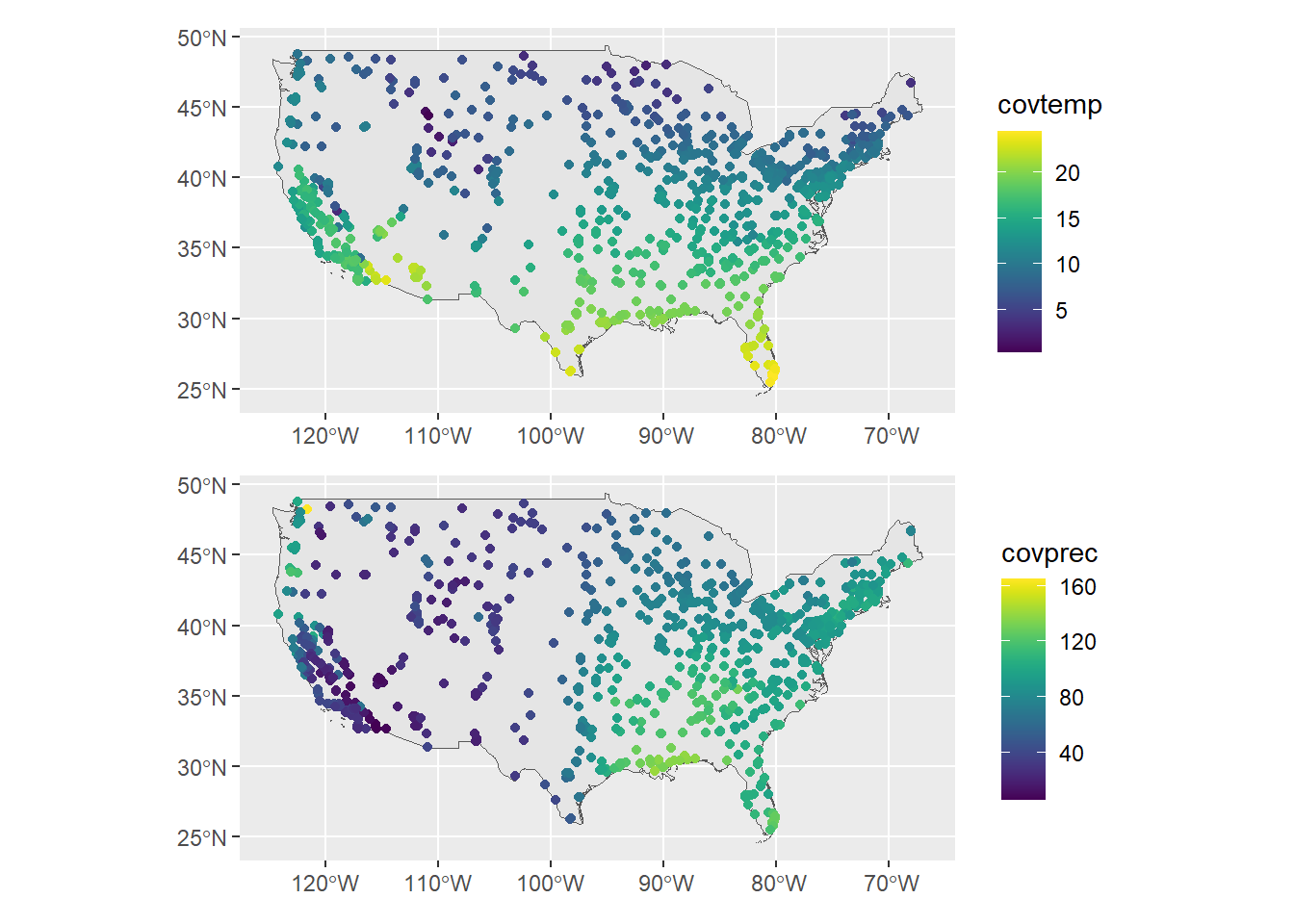
FIGURE 15.3: Temperature and precipitation measurements at the observation locations.
15.2.4 Transforming coordinates to UTM
The data we are dealing with have a geographic CRS that references locations using longitude and latitude values.
In order to work with kilometers instead of degrees,
we use st_transform() to transform the CRS of the sf objects with the data corresponding to the observed (d) and the prediction (dp) locations from geographic to a projected CRS.
Specifically, we use the Mercator projection that is given by EPSG code 3857 and use kilometers as units.
To do that, we use the projection given by st_crs("EPSG:3857")$proj4string replacing +units=m by +units=km.
st_crs("EPSG:3857")$proj4string
projMercator<-"+proj=merc +a=6378137 +b=6378137 +lat_ts=0 +lon_0=0
+x_0=0 +y_0=0 +k=1 +units=km +nadgrids=@null +wktext +no_defs"
d <- st_transform(d, crs = projMercator)
dp <- st_transform(dp, crs = projMercator)
15.2.5 Coordinates of observed and prediction locations
After transforming the data, we use the st_coordinates() function to create matrices with the projected coordinates of the observed and prediction locations.
# Observed coordinates
coo <- st_coordinates(d)

# Predicted coordinates
coop <- st_coordinates(dp)
15.2.6 Model
Now we specify the model that we use to predict PM2.5 values at unsampled locations. We assume that \(Y_i\), the PM2.5 values measured at locations \(i = 1, \ldots, n\), can be modeled as
\[Y_i \sim N(\mu_i, \sigma^2),\]
\[\mu_i = \beta_0 + \beta_1 \times \mbox{temp}_i + \beta_2 \times \mbox{prec}_i + S(\boldsymbol{x}_i),\]
where \(\beta_0\) is the intercept, and \(\beta_1\) and \(\beta_2\) are, respectively, the coefficients of temperature and precipitation. \(S(\cdot)\) is a spatial random effect that is modeled as a zero-mean Gaussian process with Matérn covariance function.
15.2.7 Mesh construction
To fit the model using the SPDE approach, we first create a triangulated mesh covering the study region where we approximate the Gaussian random field as a Gaussian Markov random field. INLA produces good approximations by using a fine mesh consisting of very small triangles and with a large separation distance between the locations and the mesh boundary to avoid boundary effects by which the variance is increased near the boundary. In some applications the use of such a fine mesh could be computationally intensive, and we usually work with meshes that still produce good approximations consisting of an inner region with small triangles where precision is needed, and an outer extension with larger triangles where accurate approximations are not needed.
Here, we create the mesh with the inla.mesh.2d() function of R-INLA. We pass as arguments loc = coo with the location coordinates, and max.edge = c(200, 500) with the maximum allowed triangle edge lengths in the region and the extension to have smaller triangles within the region than in the extension. We also specify cutoff = 1 with the minimum allowed distance between points to avoid building many small triangles in areas where locations are located close to each other (Figure 15.4).
The number of vertices of the mesh can be obtained with mesh$n, and the mesh can be plotted as follows.
   Min. 1st Qu.  Median    Mean 3rd Qu.    Max.
      0    1107    1966    2242    3311    6318
mesh <- inla.mesh.2d(loc = coo, max.edge = c(200, 500),
                     cutoff = 1)
mesh$n
[1] 3711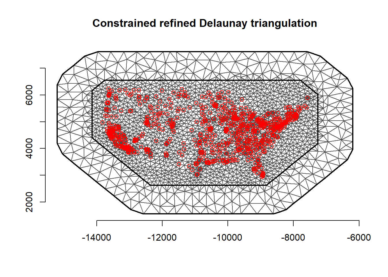
FIGURE 15.4: Mesh used in the SPDE approach. Locations of PM2.5 measurements are depicted as red points.
15.2.8 Building the SPDE on the mesh
Then, we use the inla.spde2.matern() function to build the SPDE model. This function has parameters mesh with the triangulated mesh constructed and constr = TRUE to impose an integrate-to-zero constraint. Moreover, we set the smoothness parameter \(\nu\) equal to 1. In the spatial case \(d=2\) and \(\alpha = \nu + d/2 = 2\).
spde <- inla.spde2.matern(mesh = mesh, alpha = 2, constr = TRUE)15.2.9 Index set
Then, we create an index set for the SPDE model using the inla.spde.make.index() function, where we provide the effect name (s) and the number of vertices in the SPDE model (spde$n.spde). This function generates a list with the vector s ranging from 1 to spde$n.spde. Additionally, it creates two vectors, s.group and s.repl, containing all elements set to 1 and lengths equal to the number of mesh vertices.
indexs <- inla.spde.make.index("s", spde$n.spde)
lengths(indexs)
s s.group s.repl
3711 3711 3711 15.2.10 Projection matrix
We use the inla.spde.make.A() function of R-INLA passing the mesh (mesh) and the coordinates (coo) to easily
construct a projection matrix \(A\) that projects the spatially continuous Gaussian random field from the observations to the mesh nodes.
A <- inla.spde.make.A(mesh = mesh, loc = coo)We can see the projection matrix \(A\) has a number of rows equal to the number of observations, and a number of columns equal to the number of vertices of the mesh. We also see the elements of each row of \(A\) sum to 1.
# dimension of the projection matrix
dim(A)
[1] 1366 3711
# number of observations
nrow(coo)
[1] 1366
# number of vertices of the triangulation
mesh$n
[1] 3711
# elements of each row sum to 1
# rowSums(A)
We also create a projection matrix for the prediction locations.
Ap <- inla.spde.make.A(mesh = mesh, loc = coop)15.2.11 Stack with data for estimation and prediction
We now create a stack with the data for estimation and prediction that organizes data, effects, and projection matrices.
We create stacks for estimation (stk.e) and prediction (stk.p) using tag to identify the type of data, data with the list of data vectors, A with the projection matrices, and effects with a list of fixed and random effects.
First, we create a stack named stk.e containing the data for estimation which is tagged with the string "est".
In data, we specify the response vector with the observed PM2.5 values.
The projection matrix is giving in argument A, which is a list where the second element is the projection matrix for the random effects (A) and the first element is set to 1 to indicate that the fixed effects are directly mapped one-to-one to the response.
To define the effects, we pass a list containing the fixed and random effects.
The fixed effects are a data.frame consisting of an intercept (b0) and covariates temperature (covtemp) and precipitation (covprec). The random effect is represented by the spatial Gaussian random field s containing a list with the indices of the SPDE object (indexs).
Additionally, we construct another stack called stk.p for prediction, which is labeled with the tag "pred". The data, projection matrix and effects are specified for the prediction locations.
The response vector in the argument data of this stack is set to a list with NA because these are values we want to predict.
Finally, we combine stk.e and stk.p into a single full stack named stk.full.
# stack for estimation stk.e
stk.e <- inla.stack(tag = "est",
data = list(y = d$value), A = list(1, A),
effects = list(data.frame(b0 = rep(1, nrow(A)),
covtemp = d$covtemp, covprec = d$covprec),
s = indexs))

# stack for prediction stk.p
stk.p <- inla.stack(tag = "pred",
data = list(y = NA), A = list(1, Ap),
effects = list(data.frame(b0 = rep(1, nrow(Ap)),
covtemp = dp$covtemp, covprec = dp$covprec),
s = indexs))

# stk.full has stk.e and stk.p
stk.full <- inla.stack(stk.e, stk.p)
15.2.12 Model formula and inla() call
Then, we specify the formula by including the response variable, the ~ symbol, and the fixed and random effects.
In the formula, we eliminate the intercept by adding 0 and include it as a covariate term by adding b0. This step ensures that all covariate terms are properly captured within the projection matrix.
formula <- y ~ 0 + b0 + covtemp + covprec + f(s, model = spde)Finally, we call inla() by specifying the formula, family, stack with the data, and options. We set control.predictor = list(compute = TRUE) and control.compute = list(return.marginals.predictor = TRUE) to compute and return the marginals for the linear predictor.
res <- inla(formula, family = "gaussian",
       data = inla.stack.data(stk.full),
       control.predictor = list(compute = TRUE,
                                A = inla.stack.A(stk.full)),
       control.compute = list(return.marginals.predictor = TRUE))
15.2.13 Results
A summary of the results can be inspected with summary(res). The object res$summary.fixed provides the mean and quantiles of the posterior distribution of the intercept and coefficients of the covariates.
res$summary.fixed mean sd 0.025quant 0.5quant
b0 3.883769 0.282343 3.32376 3.885582
covtemp 0.239480 0.019995 0.20106 0.239178
covprec 0.002687 0.003074 -0.00347 0.002729
0.975quant mode kld
b0 4.433450 3.885578 1.707e-08
covtemp 0.279596 0.239172 5.402e-08
covprec 0.008608 0.002729 4.568e-08We observe the coefficient of temperature is \(\hat \beta_1=\) 0.239 with a 95% credible interval equal to (0.201, 0.28). The coefficient of precipitation is \(\hat \beta_2=\) 0.003 with a 95% credible interval equal to (–0.003, 0.009). Thus, temperature is significantly associated with PM2.5, whereas precipitation is not significant.
15.2.14 Mapping predicted PM2.5 values
The res$summary.fitted.values object contains the posterior mean and quantiles of the fitted values. We can obtain the indices corresponding to the prediction locations by using the inla.stack.index() function passing the full stack and tag = "pred". Then, we retrieve the column "mean" with the posterior mean, and columns "0.025quant" and "0.975quant" with lower and upper limits of 95% credible intervals denoting the uncertainty of the predictions.
index <- inla.stack.index(stack = stk.full, tag = "pred")$data
pred_mean <- res$summary.fitted.values[index, "mean"]
pred_ll <- res$summary.fitted.values[index, "0.025quant"]
pred_ul <- res$summary.fitted.values[index, "0.975quant"]
We assign the predicted values to their corresponding cells within the map that are in the object grid that contains the prediction locations.
grid$mean <- NA
grid$ll <- NA
grid$ul <- NA

grid$mean[indicespointswithin] <- pred_mean
grid$ll[indicespointswithin] <- pred_ll
grid$ul[indicespointswithin] <- pred_ul

summary(grid) # negative values for the lower limit
mean ll ul
Min. : 2 Min. : 0 Min. : 3
1st Qu.: 6 1st Qu.: 4 1st Qu.: 7
Median : 7 Median : 5 Median : 8
Mean : 7 Mean : 5 Mean : 8
3rd Qu.: 8 3rd Qu.: 6 3rd Qu.:10
Max. :15 Max. :13 Max. :17
NA's :4189 NA's :4189 NA's :4189 Then, we plot the posterior mean and 95% credible intervals of the predicted PM2.5 values with the levelplot() function of rasterVis package.
Figure 15.5 depicts maps with the spatial pattern of the predicted PM2.5 levels as well as their associated uncertainty.
library(rasterVis)
levelplot(grid, layout = c(1, 3),
names.attr = c("Mean", "2.5 percentile", "97.5 percentile"))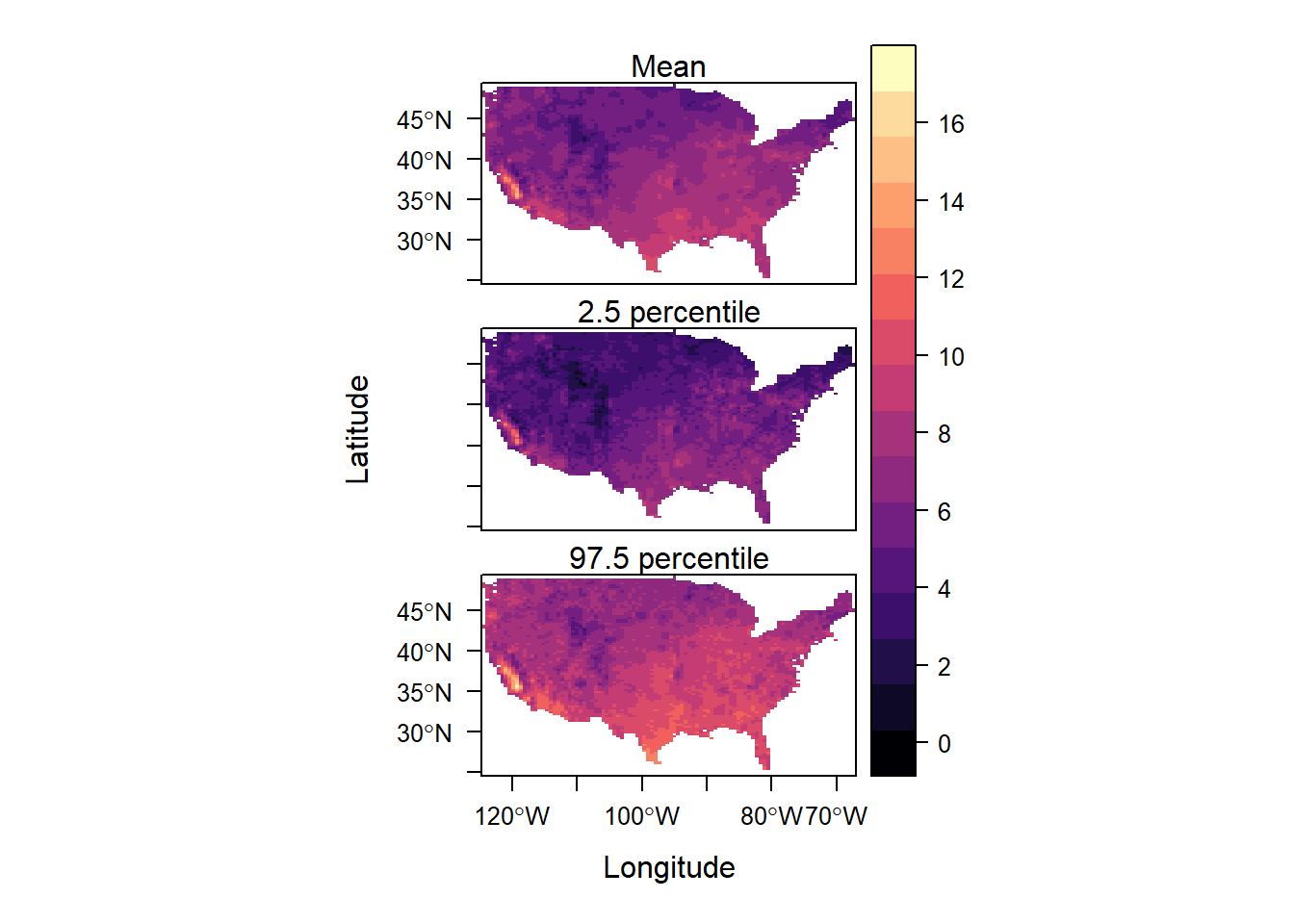
FIGURE 15.5: Posterior mean and lower and upper limits of uncertainty intervals of PM2.5.
15.2.15 Exceedance probabilities
We can also obtain probabilities that PM2.5 exceed a specific threshold level with the inla.pmarginal() function. Specifically, we calculate the probabilities that PM2.5 levels exceed 10 micrograms per cubic meter. That is, P(PM2.5 > 10) = 1 – P(PM2.5 \(\leq\) 10).
excprob <- sapply(res$marginals.fitted.values[index],
FUN = function(marg){1-inla.pmarginal(q = 10, marginal = marg)})
Then, we add the exceedance probabilities as a layer in grid, and we plot it with levelplot(). In levelplot(), we set margin = FALSE to hide the marginal graphics of the column and row summaries of the raster object.
Figure 15.6 shows the probabilities that PM2.5 levels exceed 10 micrograms per cubic meter. We observe high probabilities in the west coast and south part of the country.
grid$excprob <- NA
grid$excprob[indicespointswithin] <- excprob

levelplot(grid$excprob, margin = FALSE)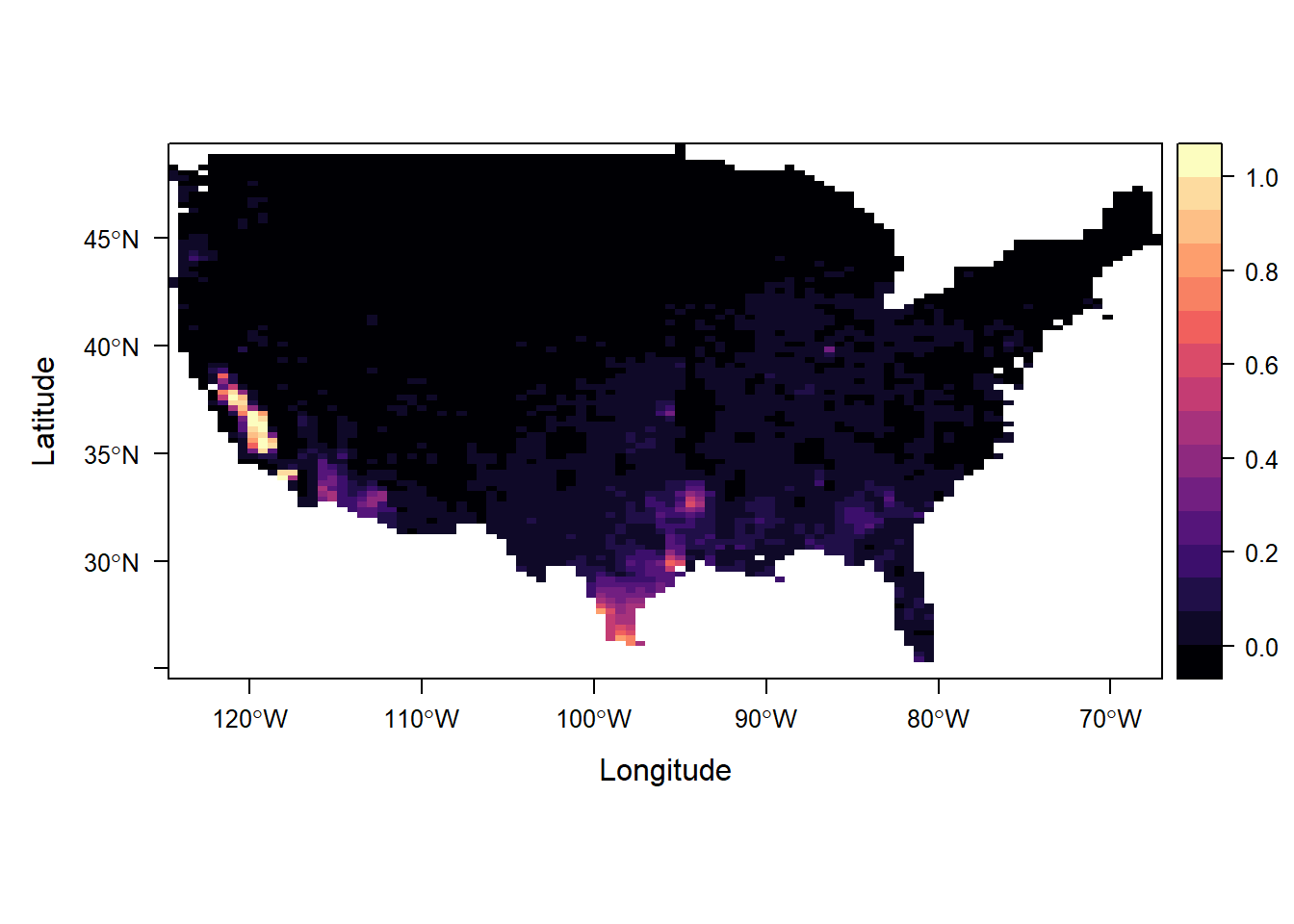
FIGURE 15.6: Probability that PM2.5 levels exceed 10 micrograms per cubic meter.