12 Building a dashboard to visualize spatial data with flexdashboard

Dashboards are tools for effective data visualization that help communicate information in an intuitive and insightful manner, and are essential to support data-driven decision making. The flexdashboard package (Aden-Buie et al. 2023) permits to create dashboards containing several related data visualization arranged on a single screen on HTML format. Visualizations can include standard R graphics and also interactive JavaScript visualizations called HTML widgets (Vaidyanathan et al. 2023).

In this chapter, we show how to create a dashboard to visualize spatial data using flexdashboard. The dashboard shows fine particulate air pollution levels (PM$_{2.5}$) in each of the world countries in 2016. Air pollution data are obtained from the World Bank using the wbstats package (Piburn 2020), and the world map is obtained from the rnaturalearth package (Massicotte and South 2023). We show how to create a dashboard that includes several interactive and static visualizations such as a map produced with leaflet (Cheng et al. 2023), a table created with DT (Xie, Cheng, and Tan 2023), and a histogram created with ggplot2 (Wickham, Chang, et al. 2023).

12.1 The R package flexdashboard

To create a dashboard with flexdashboard we need to write an R Markdown file with the extension .Rmd (Allaire et al. 2023). Chapter 11 provides an introduction to R Markdown. Here, we briefly review R Markdown, and show how to specify the layout and the components of a dashboard.

12.1.1 R Markdown

R Markdown allows easy work reproducibility by including R code that generates results and narrative text explaining the work. When the R Markdown file is compiled, the R code is executed and the results are appended to a report that can take a variety of formats including HTML and PDF documents.

An R Markdown file has three basic components, namely, YAML header, text, and R code. At the top of the R Markdown file we need to write the YAML header between a pair of three dashes ---. This header specifies several document options such as title, author, date and type of output file. To create a flexdashboard, we need to include the YAML header with the option output: flexdashboard::flex_dashboard. The text in an R Markdown file is written with Markdown syntax. For example, we can use asterisks for italic text (*text*) and double asterisks for bold text (**text**) . The R code that we wish to execute needs to be specified inside R code chunks. An R chunk starts with three backticks ```{r} and ends with three backticks ```. We can also write inline R code by writing it between `r and `.

12.1.2 Layout

Dashboard components are shown according to a layout that needs to be specified. Dashboards are divided into columns and rows. We can create layouts with multiple columns by using -------------- for each column. Dashboard components are included by using ###. Components include R chunks that contain the code needed to generate the visualizations written between ```{r} and ```. For example, the following code creates a layout with two columns with one and two components, respectively. The width of the columns is specified with the {data-width} attribute.

---
title: "Multiple Columns"
output: flexdashboard::flex_dashboard
---
    
Column {data-width=600}
-------------------------------------
    
### Component 1
    
```{r}

```
   
Column {data-width=400}
-------------------------------------
   
### Component 2

```{r}

```   
 
### Component 3
    
```{r}

```

Layouts can also be specified row-wise rather than column-wise by adding in the YAML the option orientation: rows. Additional layout examples including tabs, multiple pages and sidebars are shown in the R Markdown website.

12.1.3 Dashboard components

A flexdashboard can include a wide variety of components including the following:

Interactive JavaScript data visualizations based on HTML widgets. Examples of HTML widgets include visualizations created with the packages leaflet, DT and dygraphs. Other HTML widgets can be seen in the website https://www.htmlwidgets.org/,
Charts created with standard R graphics,
Simple tables created with knitr::kable() or interactive tables created with the DT package,
Value boxes created with the valueBox() function that display single values with a title and an icon,
Gauges that display values on a meter within a specified range,
Text, images, and equations, and
Navigation bar with links to social services, source code, or other links related to the dashboard.

12.2 A dashboard to visualize global air pollution

Here we show how to build a dashboard to show fine particulate air pollution levels (PM$_{2.5}$) in each of the world countries in 2016 (Figure 12.1). First, we explain how to obtain the data and the world map. Then we show how to create the visualizations of the dashboard. Finally, we create the dashboard by defining the layout and adding the visualizations.

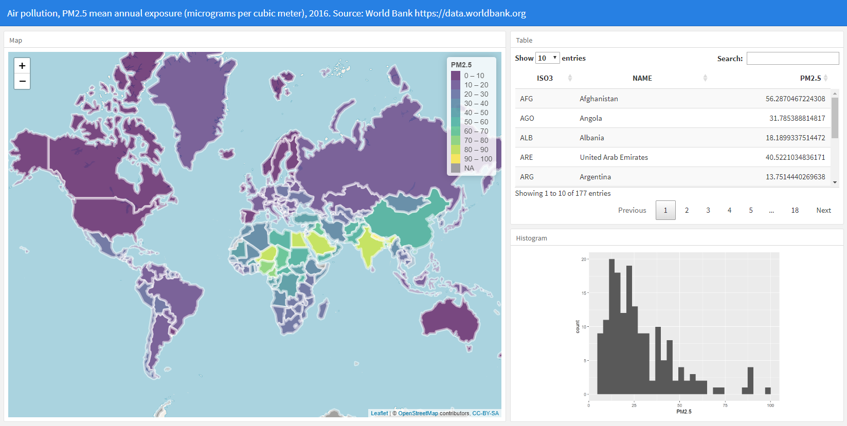
FIGURE 12.1: Snapshot of the dashboard to visualize air pollution data.

12.2.1 Data

We obtain the world map using the rnaturalearth package (Figure 12.2). Specifically, we use the ne_countries() function with the option returnclass = "sf" to obtain a sf object called map with the world country polygons. map has a variable called name with the country names, and a variable called iso_a3 with the ISO standard country codes of 3 letters. We rename these variables with names NAME and ISO3, and they will be used later to join the map with the data.

library(sf)
library(rnaturalearth)
map <- ne_countries(returnclass = "sf")
names(map)[names(map) == "iso_a3"] <- "ISO3"
names(map)[names(map) == "name"] <- "NAME"

plot(map)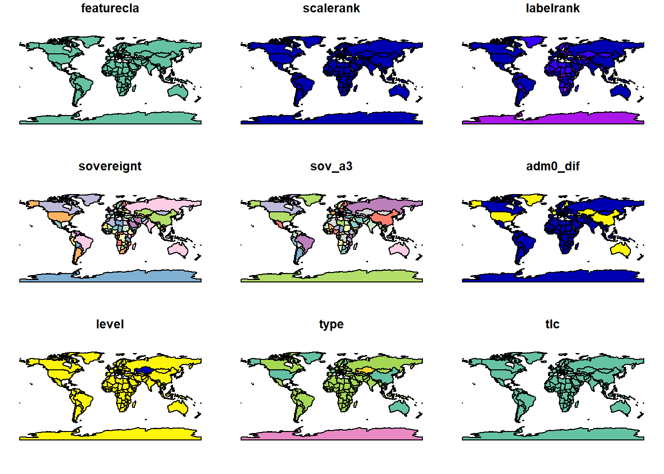

FIGURE 12.2: World map obtained from the rnaturalearth package.

We obtain PM$_{2.5}$ concentration levels using the wbstats package. This package permits to retrieve global indicators published by the World Bank. If we are interested in obtaining air pollution indicators, we can use the wb_search() function setting pattern = "pollution". This function searches all the indicators that match the specified pattern and returns a data frame with their IDs and names. We assign the search result to the object indicators that can be inspected by typing indicators.

library(wbstats)
indicators <- wb_search(pattern = "pollution")

We decide to plot the indicator PM2.5 air pollution, mean annual exposure (micrograms per cubic meter) which has code EN.ATM.PM25.MC.M3 in 2016. To download these data, we use the wb_data() function providing the indicator code and the start and end dates.

d <- wb_data(
  indicator = "EN.ATM.PM25.MC.M3",
  start_date = 2016, end_date = 2016
)
head(d)

## # A tibble: 6 × 9
##   iso2c iso3c country      date EN.ATM.PM25.MC.M3 unit 
##   <chr> <chr> <chr>       <dbl>             <dbl> <chr>
## 1 AW    ABW   Aruba        2016             NA    <NA> 
## 2 AF    AFG   Afghanistan  2016             57.2  <NA> 
## 3 AO    AGO   Angola       2016             29.2  <NA> 
## 4 AL    ALB   Albania      2016             17.8  <NA> 
## 5 AD    AND   Andorra      2016              8.94 <NA> 
## 6 AE    ARE   United Ara…  2016             43.2  <NA> 
## # ℹ 3 more variables: obs_status <chr>,
## #   footnote <chr>, last_updated <date>

The returned data frame d has a variable called value with the PM$_{2.5}$ values and a variable called iso3c with the ISO standard country codes of 3 letters. In map, we create a variable called PM2.5 with the PM$_{2.5}$ values retrieved (d$EN.ATM.PM25.MC.M3). Note that the order of the countries in the map and in the data d can be different. Therefore, when we assign d$EN.ATM.PM25.MC.M3 to the variable map$PM2.5 we need to ensure that the values added correspond to the right countries. We can use match() to calculate the positions of the ISO3 code in the map (map$ISO3) in the data (d$iso3c), and assign d$EN.ATM.PM25.MC.M3 to map$PM2.5 in that order.

map$PM2.5 <- d[match(map$ISO3, d$iso3c), ]$EN.ATM.PM25.MC.M3

We can see the first rows of map by typing head(map).

12.2.2 Table using DT

Now we create the visualizations that will be included in the dashboard. First, we create an interactive table that shows the data by using the DT package (Figure 12.3). We use the datatable() function to show a data frame with variables ISO3, NAME, and PM2.5. We set rownames = FALSE to hide row names, and options = list(pageLength = 10) to set the page length equal to 10 rows. The table created enables filtering and sorting of the variables shown.

library(DT)
DT::datatable(map[, c("ISO3", "NAME", "PM2.5")],
  rownames = FALSE, options = list(pageLength = 10)
)

FIGURE 12.3: Table with the PM$_{2.5}$ values.

12.2.3 Map using leaflet

Next, we create an interactive map with the PM$_{2.5}$ values of each country by using the leaflet package (Figure 12.4). To color the countries according to their PM$_{2.5}$ values, we first create a color palette. We call this palette pal and create it by using the colorNumeric() function with argument palette equal to viridis, domain equal to the PM$_{2.5}$ values, and cut points equal to the sequence from 0 to the maximum PM$_{2.5}$ values in increments of 10. To create the map, we use the leaflet() function passing the map object. We write addTiles() to add a background map, and add setView() to center and zoom the map. Then we use addPolygons() to plot the areas of the map. We color the areas with the colors given by the PM$_{2.5}$ values and the palette pal. In addition, we color the border of the areas (color) with color white and set fillOpacity = 0.7 so the background map can be seen. Finally we add a legend with the function addLegend() specifying the color palette, values, opacity and title.

We also wish to show labels with the name and PM$_{2.5}$ levels of each of the countries. We can create the labels using HTML code and then apply the HTML() function of the htmltools package so leaflet knows how to plot them. Then we add the labels to the argument label of addPolygons(), and add highlight options to highlight areas as the mouse passes over them.

library(leaflet)

pal <- colorBin(
  palette = "viridis", domain = map$PM2.5,
  bins = seq(0, max(map$PM2.5, na.rm = TRUE) + 10, by = 10)
)


map$labels <- paste0(
  "<strong> Country: </strong> ",
  map$NAME, "<br/> ",
  "<strong> PM2.5: </strong> ",
  map$PM2.5, "<br/> "
) %>%
  lapply(htmltools::HTML)

leaflet(map) %>%
  addTiles() %>%
  setView(lng = 0, lat = 30, zoom = 2) %>%
  addPolygons(
    fillColor = ~ pal(PM2.5),
    color = "white",
    fillOpacity = 0.7,
    label = ~labels,
    highlight = highlightOptions(
      color = "black",
      bringToFront = TRUE
    )
  ) %>%
  leaflet::addLegend(
    pal = pal, values = ~PM2.5,
    opacity = 0.7, title = "PM2.5"
  )

FIGURE 12.4: Leaflet map with the PM$_{2.5}$ values.

12.2.4 Histogram using ggplot2

We also create a histogram with the PM$_{2.5}$ values using the ggplot() function of the ggplot2 package (Figure 12.5).

library(ggplot2)
ggplot(data = map, aes(x = PM2.5)) + geom_histogram()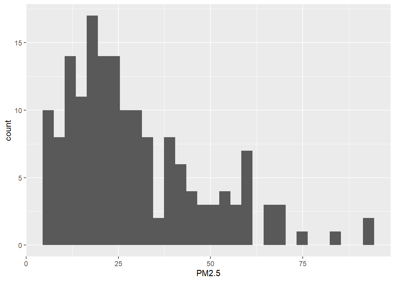

$Histogram of the PM$_{2.5}$ values.$

FIGURE 12.5: Histogram of the PM$_{2.5}$ values.

12.2.5 R Markdown structure. YAML header and layout

Now we write the structure of the R Markdown document. In the YAML header, we specify the title and the type of output file (flexdashboard::flex_dashboard). We create a dashboard with two columns with one and two rows, respectively. Columns are created by using --------------, and the components are included by using ###. We set the width of the first column to 600 pixels, and the second column to 400 pixels using the {data-width} attribute. We write an R chunk for the leaflet map in the first column, and R chunks for the table and the histogram in the second column.

---
title: "Air pollution, PM2.5 mean annual exposure 
  (micrograms per cubic meter), 2016"
  Source: World Bank https://data.worldbank.org"
output: flexdashboard::flex_dashboard
---
    
Column {data-width=600}
-------------------------------------
    
### Map
    
```{r}

```
   
Column {data-width=400}
-------------------------------------
   
### Table

```{r}

```   
 
### Histogram
    
```{r}

```

12.2.6 R code to obtain the data and create the visualizations

We finish the dashboard by adding the R code needed to obtain the data and create the visualizations. Below the YAML code, we add an R chunk with the code to load the packages needed, and obtain the map and the PM$_{2.5}$ data. Then, in the corresponding components, we add R chunks with the code to create the map, the table and the histogram. Finally, we compile the R Markdown file and obtain the dashboard that shows global PM$_{2.5}$ levels in 2016. A snapshot of the dashboard created is shown in Figure 12.1. The complete code to create the dashboard is the following:

---
title: "Air pollution, PM2.5 mean annual exposure
  (micrograms per cubic meter), 2016.
  Source: World Bank https://data.worldbank.org"
output: flexdashboard::flex_dashboard
---


```{r}
library(sf)
library(rnaturalearth)
library(wbstats)
library(leaflet)
library(DT)
library(ggplot2)

map <- ne_countries(returnclass = "sf")
names(map)[names(map) == "iso_a3"] <- "ISO3"
names(map)[names(map) == "name"] <- "NAME"

d <- wb_data(
  indicator = "EN.ATM.PM25.MC.M3",
  start_date = 2016, end_date = 2016
)

map$PM2.5 <- d[match(map$ISO3, d$iso3c), ]$EN.ATM.PM25.MC.M3
```
  
  
Column {data-width=600}
-------------------------------------

### Map


```{r}
pal <- colorBin(
  palette = "viridis", domain = map$PM2.5,
  bins = seq(0, max(map$PM2.5, na.rm = TRUE) + 10, by = 10)
)

map$labels <- paste0(
  "<strong> Country: </strong> ",
  map$NAME, "<br/> ",
  "<strong> PM2.5: </strong> ",
  map$PM2.5, "<br/> "
) %>%
  lapply(htmltools::HTML)

leaflet(map) %>%
  addTiles() %>%
  setView(lng = 0, lat = 30, zoom = 2) %>%
  addPolygons(
    fillColor = ~ pal(PM2.5),
    color = "white",
    fillOpacity = 0.7,
    label = ~labels,
    highlight = highlightOptions(
      color = "black",
      bringToFront = TRUE
    )
  ) %>%
  leaflet::addLegend(
    pal = pal, values = ~PM2.5,
    opacity = 0.7, title = "PM2.5"
  )
```
   

Column {data-width=400}
-------------------------------------

### Table


```{r}
DT::datatable(map[, c("ISO3", "NAME", "PM2.5")],
  rownames = FALSE, options = list(pageLength = 10)
)
```   

### Histogram


```{r}
ggplot(data = map, aes(x = PM2.5)) + geom_histogram()
```

11 Introduction to R Markdown

13 Introduction to Shiny