11 Introduction to R Markdown

R Markdown (Allaire et al. 2024) can be used to easily turn our analysis into fully reproducible documents that can be shared with others to communicate our analysis quickly and effectively. An R Markdown file is written with Markdown syntax with embedded R code, and can include narrative text, tables and visualizations. When an R Markdown file is compiled, the R code is executed and the results are automatically appended to a document that can take a variety of formats including HTML and PDF. In this chapter, we give an introduction to R Markdown and show how to use it to generate a report that shows the results of a simple analysis of data from the package gapminder (Bryan 2023) by means of several plots, tables and narrative text.

11.1 R Markdown

We can install the rmarkdown package by typing install.packages("rmarkdown"). An R Markdown file has .Rmd extension and intermingles R code with text to create a final output in HTML, PDF or other formats. An R Markdown file has three basic components, namely:

YAML header specifying several document options such as the output format,
text written with Markdown syntax,
R code chunks with the code that needs to be executed.

To generate a document from the .Rmd file, we can use the ‘Knit’ button in the RStudio IDE or use the render() function of the rmarkdown package. The render() function has an argument called output_format where we can select the format we want for the final document. For example, we can obtain a document with HTML format if we set output_format=html_document, or a document with PDF format by setting output_format=pdf_document.

When the .Rmd file is rendered, the knit() function of the package knitr (Xie 2023) is used to execute the R code chunks and to generate a markdown file (with extension .md) that includes the code and the output. Then, Pandoc (http://pandoc.org) is used to transform the markdown file into formatted text and to create the final document in the specified format.

Below we describe the components of R Markdown in more detail. Further information about R Markdown can be seen in Xie, Allaire, and Grolemund (2018), the R Markdown website, and the R Markdown reference guide.

11.2 YAML

At the top of the R Markdown file, we need to write the YAML header between a pair of three dashes ---. This header specifies several document options such as title, author, date and type of output file. A basic YAML where the output format is set to PDF is the following:

---
title: "An R Markdown document"
author: "Paula Moraga"
date: "1 July 2019"
output: pdf_document
---

Other YAML options include the following:

fontsize to specify the font size,
toc: true to include a table of contents (TOC) at the start of the document,
toc_depth: n to specify that the lowest level of headings to add to the table of contents is given by the number n.

For example, the YAML below specifies an HTML document with font size 12pt, and includes a table of contents where 2 is the lowest level of headings. The date of the report is set to the current date by writing the inline R expression `r Sys.Date()`.

---
title: "An R Markdown document"
author: "Paula Moraga"
date: "`r Sys.Date()`"
fontsize: 12pt
output:
  html_document:
    toc: true
    toc_depth: 2
---

11.3 Markdown syntax

The text in an R Markdown file is written with Markdown syntax. Markdown is a lightweight markup language that creates styled text using a lightweight plain text syntax. For example, we can use asterisks to generate italic text and double asterisks to generate bold text.

*italic text*

italic text

**bold text**

bold text

We can mark text as inline code by writing it between a pair of backticks.

`x+y`

x+y

To start a new pararaph, we can end a line with two or more spaces. We can also write section headers using pound signs (#, ## and ### for first, second and third level headers, respectively).

# First-level header

## Second-level header

### Third-level header

Lists with unordered items can be written with -, *, or +, and lists with ordered list items can be written with numbers. Lists can be nested by indenting the sublists.

- unordered item
- unordered item
    1. first item
    2. second item
    3. third item

unordered item
unordered item
1. first item
2. second item
3. third item

We can also write math formulas using LaTex syntax.

$$\int_0^\infty e^{-x^2} dx=\frac{\sqrt{\pi}}{2}$$

\[\int_0^\infty e^{-x^2} dx=\frac{\sqrt{\pi}}{2}\]

Hyperlinks can be added using the syntax [text](link). For example, a hyperlink to the R Markdown website can be created as follows:

[R Markdown](https://rmarkdown.rstudio.com/)

R Markdown

11.4 R code chunks

The R code that we wish to execute needs to be specified inside an R code chunk. An R chunk starts with three backticks ```{r} and ends with three backticks ```. We can also write inline R code by writing it between `r and `. We can specify the behavior of a chunk by adding options in the first line between the braces and separated by commas. For example, if we use

echo=FALSE the code will not be shown in the document, but it will run and the output will be displayed in the document,
eval=FALSE the code will not run, but it will be shown in the document,
include=FALSE the code will run, but neither the code nor the output will be included in the document,
results='hide' the output will not be shown, but the code will run and will be displayed in the document.

Sometimes, the R code produces messages we do not want to include in the final document. To supress them, we can use

error=FALSE to supress errors,
warning=FALSE to supress warnings,
message=FALSE to supress messages.

In addition, if we wish to use certain options frequently, we can set these options globally in the first code chunk. Then, if we want particular chunks to behave differently, we can specify different options for them. For example, we can supress the R code and the messages in all chunks of the document as follows:

```{r, include=FALSE}
knitr::opts_chunk$set(echo=FALSE, message=FALSE)
```

Below, we show an R code chunk that loads the gapminder package and attaches the gapminder data that contains data of life expectancy, gross domestic product (GDP) per capita (US$, inflation-adjusted), and population by country from 1952 to 2007. Then it shows its first elements with head(gapminder) and a summary with summary(gapminder). The chunk includes an option to supress warnings.

```{r, warning=FALSE}
library(gapminder)
data(gapminder)
head(gapminder)
summary(gapminder)
```

## # A tibble: 6 × 6
##   country     continent  year lifeExp     pop gdpPercap
##   <fct>       <fct>     <int>   <dbl>   <int>     <dbl>
## 1 Afghanistan Asia       1952    28.8  8.43e6      779.
## 2 Afghanistan Asia       1957    30.3  9.24e6      821.
## 3 Afghanistan Asia       1962    32.0  1.03e7      853.
## 4 Afghanistan Asia       1967    34.0  1.15e7      836.
## 5 Afghanistan Asia       1972    36.1  1.31e7      740.
## 6 Afghanistan Asia       1977    38.4  1.49e7      786.

##         country        continent        year     
##  Afghanistan:  12   Africa  :624   Min.   :1952  
##  Albania    :  12   Americas:300   1st Qu.:1966  
##  Algeria    :  12   Asia    :396   Median :1980  
##  Angola     :  12   Europe  :360   Mean   :1980  
##  Argentina  :  12   Oceania : 24   3rd Qu.:1993  
##  Australia  :  12                  Max.   :2007  
##  (Other)    :1632                                
##     lifeExp          pop             gdpPercap     
##  Min.   :23.6   Min.   :6.00e+04   Min.   :   241  
##  1st Qu.:48.2   1st Qu.:2.79e+06   1st Qu.:  1202  
##  Median :60.7   Median :7.02e+06   Median :  3532  
##  Mean   :59.5   Mean   :2.96e+07   Mean   :  7215  
##  3rd Qu.:70.8   3rd Qu.:1.96e+07   3rd Qu.:  9325  
##  Max.   :82.6   Max.   :1.32e+09   Max.   :113523  
##

Other possible Markdown syntax specifications and R chunks options can be explored in the R Markdown reference guide.

11.5 Figures

Figures can be created by writing the R code that generates them inside an R code chunk. In the R chunk we can write the option fig.cap to write a caption, and fig.align to specify the alignment of the figure ('left', 'center' or 'right'). We can also use out.width and out.height to specify the size of the output. For example, out.width = '80%' means the output occupies 80% of the page width.

The following chunk creates a scatterplot with life expectancy at birth versus GDP per capita in 2007 obtained from the gapminder data (Figure 11.1). The chunk uses fig.cap to specify a caption for the figure.

```{r, fig.cap='Life expectancy versus GDP per capita in 2007.'}
library(ggplot2)
ggplot(
  gapminder[which(gapminder$year == 2007), ],
  aes(x = gdpPercap, y = lifeExp)
) +
  geom_point() +
  xlab("GDP per capita (US$)") +
  ylab("Life expectancy (years)")
```

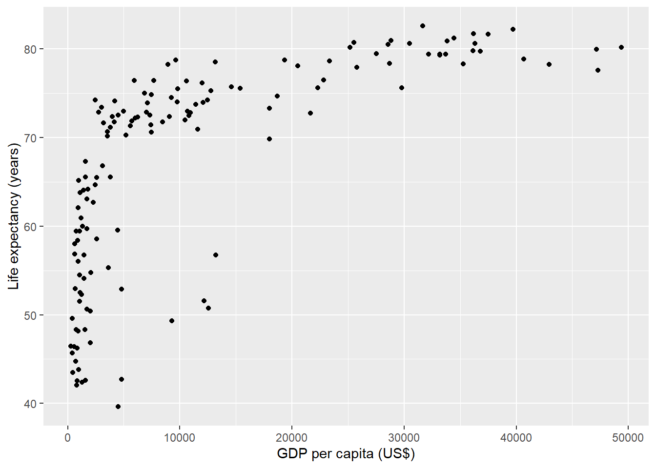
FIGURE 11.1: Life expectancy versus GDP per capita in 2007.

Images that are already saved can also be easily included with Markdown syntax. For example, if the image is saved in path path/img.png, it can be included in the document using

![optional caption text](path/img.png)

We can also include the image with the include_graphics() function of the knitr package. This allows to specify chunk options. For example, we can include a centered figure that occupies 25% of the document and has caption Figure 1 as follows:

```{r, out.width='25%', fig.align='center', fig.cap='Figure 1'}
knitr::include_graphics("path/img.png")
```

11.6 Tables

Tables can be included with the kable() function of the knitr package. kable() has an argument called caption to add a caption to the table produced. The code below shows the code to create a table with the first rows of the gapminder data (Table 11.1).

```{r}
knitr::kable(head(gapminder),
  caption = "First rows of the 'gapminder' data."
)
```

TABLE 11.1: First rows of the `gapminder’ data.
country	continent	year	lifeExp	pop	gdpPercap
Afghanistan	Asia	1952	28.80	8425333	779.4
Afghanistan	Asia	1957	30.33	9240934	820.9
Afghanistan	Asia	1962	32.00	10267083	853.1
Afghanistan	Asia	1967	34.02	11537966	836.2
Afghanistan	Asia	1972	36.09	13079460	740.0
Afghanistan	Asia	1977	38.44	14880372	786.1

In addition, we can use the kableExtra package (Zhu 2024) to manipulate table styles and to easily build common complex tables. For example, we can use the kable_styling() function to adjust the size of tables in PDF documents or add scrollbars in tables of HTML documents.

11.7 Example

Here we show how to create an R Markdown report with a simple analysis of the gapminder data in 2007. The document includes a table with a summary of the data and a scatterplot of life expectancy versus GDP, as well as the R code that generates these outputs. The report is generated in PDF format. To create this report, we first open a new .Rmd file and write a YAML header with the title, author, date and specifying PDF output. Then we write R code chunks to generate the visualizations intermingled with text explaining the data, code and our conclusions. Specifically, we include a table with the summary of the data corresponding to 2007 using the kable() function.

library(gapminder)
library(kableExtra)
data(gapminder)
d <- gapminder[which(gapminder$year == 2007), ]
knitr::kable(summary(d),
  caption = "Summary of the `gapminder` data in 2007."
)

TABLE 11.2: Summary of the `gapminder` data in 2007.
country	continent	year	lifeExp	pop	gdpPercap
Afghanistan: 1	Africa :52	Min. :2007	Min. :39.6	Min. :2.00e+05	Min. : 278
Albania : 1	Americas:25	1st Qu.:2007	1st Qu.:57.2	1st Qu.:4.51e+06	1st Qu.: 1625
Algeria : 1	Asia :33	Median :2007	Median :71.9	Median :1.05e+07	Median : 6124
Angola : 1	Europe :30	Mean :2007	Mean :67.0	Mean :4.40e+07	Mean :11680
Argentina : 1	Oceania : 2	3rd Qu.:2007	3rd Qu.:76.4	3rd Qu.:3.12e+07	3rd Qu.:18009
Australia : 1	NA	Max. :2007	Max. :82.6	Max. :1.32e+09	Max. :49357
(Other) :136	NA	NA	NA	NA	NA

Then, we create a scatterplot of life expectancy versus GDP of the world countries in 2007 using the ggplot() function of the ggplot2 package. Each of the points of the plot represents a country. Points are colored by continent and have size proportional to their population. In ggplot() we set alpha to 0.5 to make the points transparent to avoid overplotting (Figure 11.2).

library(ggplot2)
g <- ggplot(d, aes(
  x = gdpPercap, y = lifeExp,
  color = continent, size = pop, ids = country
)) +
  geom_point(alpha = 0.5) +
  ggtitle("Life expectancy versus GDP, 2007") +
  xlab("GDP per capita (US$)") +
  ylab("Life expectancy (years)") +
  scale_color_discrete(name = "Continent") +
  scale_size_continuous(name = "Population")
g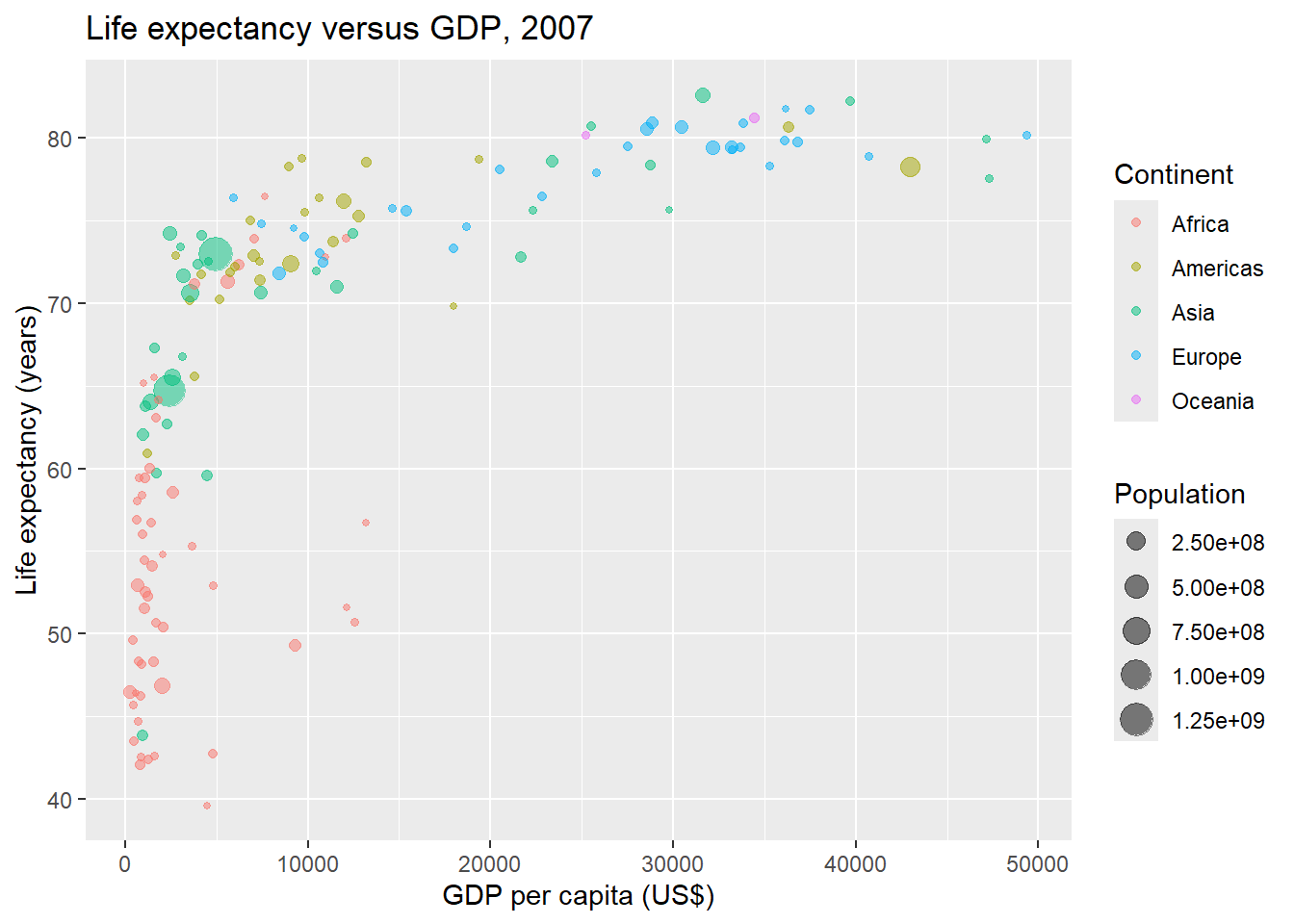

FIGURE 11.2: Life expectancy versus GDP per capita in 2007 created with ggplot2.

We also create an interactive plot with the ggplotly() function of the plotly package by just passing the ggplot object to the ggplotly() function. The ggplot object has ids = country, and the tooltip of the plotly object displays country in addition to the other values.

library(plotly)
ggplotly(g)

FIGURE 11.3: Life expectancy versus GDP per capita in 2007 created with plotly.

Finally, we render the document by clicking the ‘Knit’ button on RStudio (or using the render() function) and obtain the final PDF document. This document can be shared with others to show our code and results. Below is the complete code of the R Markdown document. At the beginning of the document we write an R chunk where to globally supress warnings and messages using knitr::opts_chunk$set().

---
title: "Life expectancy and GDP data in the world, 2007."
author: "Paula Moraga"
date: "`r Sys.Date()`"
output: pdf_document
---


```{r}
knitr::opts_chunk$set(warning=FALSE, message=FALSE)
```

# Introduction

This report shows several visualizations of the life expectancy
and GDP of the world countries in 2007.

# Data

Data are obtained from the **gapminder** package. A summary of
the data corresponding to 2007 is shown in the table below.

```{r}
library(gapminder)
data(gapminder)
d <- gapminder[which(gapminder$year == 2007), ]
knitr::kable(summary(d),
  caption = "Summary of the gapminder data in 2007"
)
```

# Visualizations

We use the `ggplot()` function of the package **ggplot2** to
create a scatterplot of life expectancy versus GDP of the world
countries in 2007. Each of the points of the plot represents
a country. Points are colored by continent and have size
proportional to their population.
In `ggplot()` we set `alpha` to 0.5 to make the points
transparent to avoid overplotting.

```{r, fig.cap='Life expectancy versus GDP per capita in 2007'}
library(ggplot2)
library(ggplot2)

g <- ggplot(d, aes(
  x = gdpPercap, y = lifeExp,
  color = continent, size = pop, ids = country
)) +
  geom_point(alpha = 0.5) +
  ggtitle("Life expectancy versus GDP, 2007") +
  xlab("GDP per capita (US$)") +
  ylab("Life expectancy (years)") +
  scale_color_discrete(name = "Continent") +
  scale_size_continuous(name = "Population")
g
``` 

This plot can be made interactive with the `ggplotly()` function
of the **plotly** package by just passing the `ggplot` object to
the `ggplotly()` function.
Note that the `ggplot` object had `ids = country` and the tooltip
of the `plotly` object displays the country in addition to the
other values.


```{r, fig.cap='Life expectancy versus GDP per capita in 2007.'}
library(plotly)
ggplotly(g)
```

# Conclusion

We have visually showed that people in countries with a high
GDP per capita live longer, and there is a big difference in
life expectancy between countries of the same income level.

10 Spatio-temporal modeling of geostatistical data. Air pollution in Spain

12 Building a dashboard to visualize spatial data with flexdashboard