16 Disease surveillance with SpatialEpiApp
SpatialEpiApp (R-SpatialEpiApp?) is an R package that contains a Shiny web application to visualize spatial and spatio-temporal disease data, estimate disease risk and detect clusters. SpatialEpiApp may be useful for many researchers and practitioners working in public health and lacking the adequate statistical and programming skills to effectively use the statistical software required to conduct disease surveillance analyses. With SpatialEpiApp, users simply need to upload a map and disease data, and then click the buttons that create the input files required, analyze the data, and process the output to generate tables and plots with the results.
SpatialEpiApp allows to fit Bayesian hierarchical models to obtain disease risk estimates and their uncertainty by using R-INLA (Havard Rue, Lindgren, and Teixeira Krainski 2024), and to detect clusters by using the scan statistics implemented in the SaTScan software (Kulldorff 2006).
Moreover, the application allows user interaction and includes interactive visualizations by using the packages leaflet for rendering maps (Cheng et al. 2024), dygraphs for plotting time series
(Vanderkam et al. 2018), and DT for displaying data objects (Xie, Cheng, and Tan 2024). It also enables the generation of reports containing the analyses performed by using R Markdown (Allaire et al. 2024).
In this chapter we describe the main components of SpatialEpiApp. Moraga (2017) can be seen for more details about its use, methods and examples.
16.1 Installation
The development version of SpatialEpiApp can be installed from GitHub by using the install_github() function of the devtools package (Wickham et al. 2022).
library(devtools)
install_github("Paula-Moraga/SpatialEpiApp")
Then, the application can be launched by loading the package and executing the run_app() function.
library(SpatialEpiApp)
run_app()
16.2 Use of SpatialEpiApp
SpatialEpiApp consists of three pages, namely, ‘Inputs’, ‘Analysis’ and ‘Help’.
16.2.1 ‘Inputs’ page
The ‘Inputs’ page is the first page we see when we launch the application (Figure 16.1). In this page we can upload the map and the disease data, and select the type of analysis to be conducted.
- The map is a shapefile with the areas of the study region. The shapefile needs to contain the id and the name of the areas.
- The data is a CSV file that contains the cases and population for each area, time, and individual level covariates (e.g., age, sex). If areal level covariates are used, the data need to specify the cases and population for each area and time, and the values of the covariates (e.g., socio-economic index).
Note that the ids of the areas in the CSV file need to be the same as the ids of the areas in the shapefile so that the data and the map can be linked. Time can be year, month or day, and all dates need to be consecutive. For example, if we work with years from 2000 to 2010, we need to provide information of all years 2000, 2001, 2002, \(\ldots\) 2010. The application does not work if we have, for example, only years 2000, 2005 and 2010. Once we have uploaded the map and the data, we need to select the type of analysis by specifying the temporal unit, the date range, and the type of analysis which can be spatial or spatio-temporal.
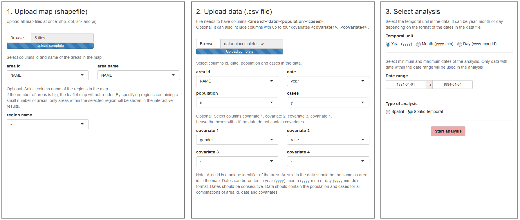
FIGURE 16.1: ‘Inputs’ page of SpatialEpiApp.
16.2.2 ‘Analysis’ page
In the ‘Analysis’ page, we can visualize the data, perform the statistical analyses, and generate reports (Figure 16.2). On the top of the page, there are four buttons:
- ‘Edit Inputs’ which is used when we wish to return to the ‘Inputs’ page to modify the analysis options or upload new data,
- ‘Maps Pop O E SIR’ which creates plots of the population, observed, expected and SIR variables,
- ‘Estimate Risk’ which is used to estimate the disease risk and its uncertainty,
- ‘Detect Clusters’ which is used for the detection of disease clusters.
To obtain disease risk estimates, we need to install the R-INLA package.
To detect clusters, we need to download and install the SaTScan software from http://www.satscan.org.
Then we need to locate the folder where the SaTScan software is installed and copy the SaTScanBatch64 executable in the SpatialEpiApp/SpatialEpiApp/ss folder which is located in the R library path. Note that the R library path can be obtained by typing .libPaths().
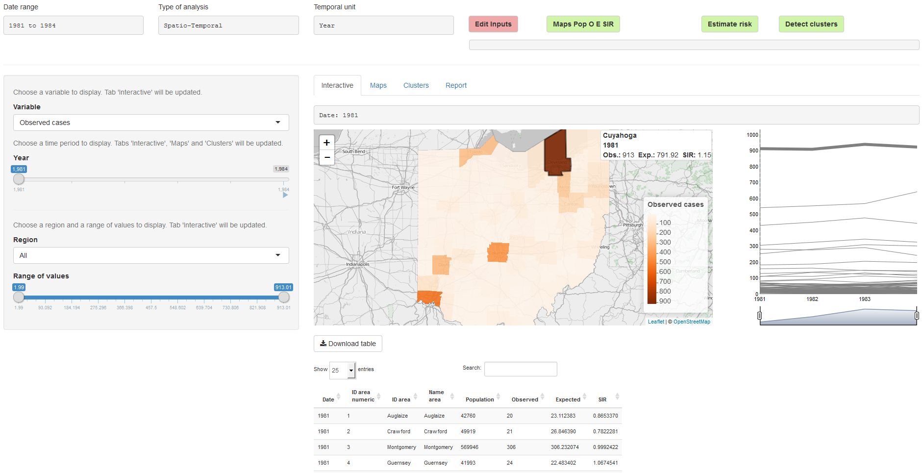
FIGURE 16.2: ‘Analysis’ page of SpatialEpiApp.
The ‘Analysis’ page also contains four tabs called ‘Interactive’, ‘Maps’, ‘Clusters’ and ‘Report’ that include tables and plots with the results. The ‘Maps’ tab (Figure 16.3) shows the results obtained by clicking the ‘Map Pop O E SIR’ and the ‘Estimate Risk’ buttons. Specifically, it shows a summary table, maps, and time plots of the population, observed number of cases, expected number of cases, SIR, disease risk, and lower and upper limits of 95% credible intervals.
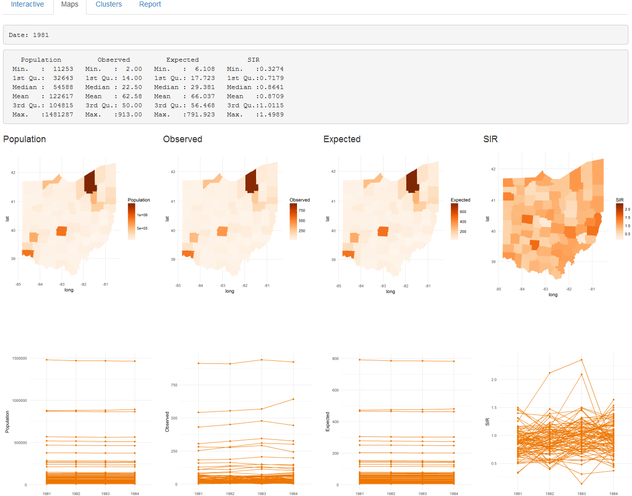
FIGURE 16.3: ‘Maps’ tab of SpatialEpiApp.
The ‘Clusters’ tab (Figure 16.4) shows the results of the cluster analysis. Specifically, it shows a map with the clusters detected for each of the times of the study period, and a plot with all clusters over time. This tab also includes a table with the information relative to each of the clusters, such as the areas that form the clusters and their significance.
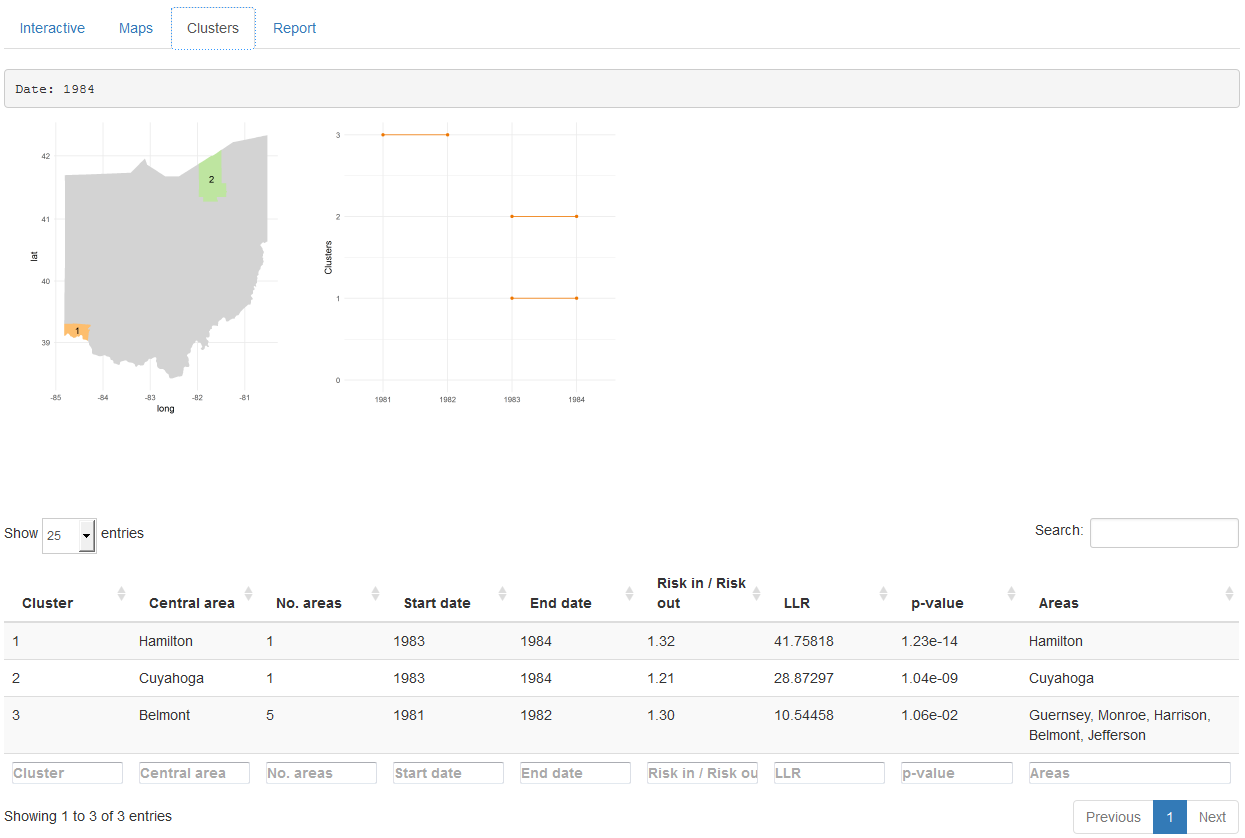
FIGURE 16.4: ‘Clusters’ tab of SpatialEpiApp.
In the ‘Report’ tab (Figure 16.5), we can download a PDF document with the results of our analysis. The report includes maps and tables summarizing the population, observed number of cases, expected number of cases, SIR, disease risk, and lower and upper limits of the 95% credible intervals, as well as the clusters detected.
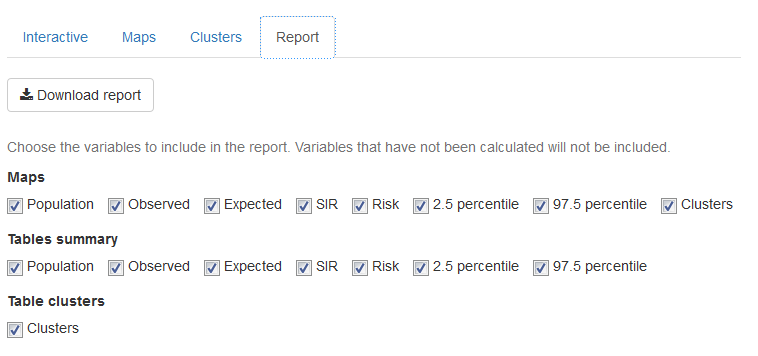
FIGURE 16.5: ‘Report’ tab of SpatialEpiApp.