4 The R-INLA package

The integrated nested Laplace approximation (INLA) approach is implemented in the R package R-INLA (Havard Rue, Lindgren, and Teixeira Krainski 2023). Instructions to download the package are given on the INLA website (http://www.r-inla.org) which also includes documentation about the package, examples, a discussion forum, and other resources about the theory and applications of INLA. The package R-INLA is not on CRAN (the Comprehensive R Archive Network) because it uses some external C libraries that make difficult to build the binaries. Therefore, when installing the package, we need to use install.packages() adding the URL of the R-INLA repository. For example, to install the stable version of the package, we need to type the following instruction:

install.packages("INLA",
repos = "https://inla.r-inla-download.org/R/stable", dep = TRUE)

Then, to load the package in R, we need to type

library(INLA)

To fit a model using INLA we need to take two steps. First, we write the linear predictor of the model as a formula object in R. Then, we run the model calling the inla() function where we specify the formula, the family, the data and other options. The execution of inla() returns an object that contains the information of the fitted model including several summaries and the posterior marginals of the parameters, the linear predictors, and the fitted values. These posteriors can then be post processed using a set of functions provided by R-INLA. The package also provides estimates of different criteria to assess and compare Bayesian models. These include the model deviance information criterion (DIC) (Spiegelhalter et al. 2002), the Watanabe-Akaike information criterion (WAIC) (Watanabe 2010), the marginal likelihood, and the conditional predictive ordinates (CPO) (Held, Schrödle, and Rue 2010). Further details about the use of R-INLA are given below.

4.1 Linear predictor

The syntax of the linear predictor in R-INLA is similar to the syntax used to fit linear models with the lm() function. We need to write the response variable, then the ~ symbol, and finally the fixed and random effects separated by + operators. Random effects are specified by using the f() function. The first argument of f() is an index vector that specifies the element of the random effect that applies to each observation, and the second argument is the name of the model (e.g., "iid", "ar1"). Additional parameters of f() can be seen by typing ?f. For example, if we have the model

\[Y_i \sim N(\eta_i, \sigma^2),\ i = 1,\ldots,n,\]

\[\eta_i = \beta_0 + \beta_1 x_1 + \beta_2 x_2 + u_i,\] where \(Y_i\) is the response variable, \(\eta_i\) is the linear predictor, \(x_1\), \(x_2\) are two explanatory variables, and \(u_i \sim N(0, \sigma_u^2)\), the formula is written as

y ~ x1 + x2 + f(i, model = "iid")

Note that by default the formula includes an intercept. If we wanted to explicitly include \(\beta_0\) in the formula, we would need to remove the intercept (adding 0) and include it as a covariate term (adding b0).

y ~ 0 + b0 + x1 + x2 + f(i, model = "iid")

4.2 The inla() function

The inla() function is used to fit the model. The main arguments of inla() are the following:

• formula: formula object that specifies the linear predictor,
• data: data frame with the data. If we wish to predict the response variable for some observations, we need to specify the response variable of these observations as NA,
• family: string or vector of strings that indicate the likelihood family such as gaussian, poisson or binomial. By default family is gaussian. A list of possible alternatives can be seen by typing names(inla.models()$likelihood), and details for individual families can be seen with inla.doc("familyname"),
• control.compute: list with the specification of several computing variables such as dic which is a Boolean variable indicating whether the DIC of the model should be computed,
• control.predictor: list with the specification of several predictor variables such as link which is the link function of the model, and compute which is a Boolean variable that indicates whether the marginal densities for the linear predictor should be computed.

4.3 Priors specification

The names of the priors available in R-INLA can be seen by typing names(inla.models()$prior), and a list with the options of each of the priors can be seen with inla.models()$prior. The documentation regarding a specific prior can be seen with inla.doc("priorname").

By default, the intercept of the model is assigned a Gaussian prior with mean and precision equal to 0. The rest of the fixed effects are assigned Gaussian priors with mean equal to 0 and precision equal to 0.001. These values can be seen with inla.set.control.fixed.default()[c("mean.intercept", "prec.intercept", "mean", "prec")]. The values of these priors can be changed in the control.fixed argument of inla() by assigning a list with the mean and precision of the Gaussian distributions. Specifically, the list contains mean.intercept and prec.intercept which represent the prior mean and precision for the intercept, and mean and prec which represent the prior mean and precision for all fixed effects except the intercept.

prior.fixed <- list(mean.intercept = <>, prec.intercept = <>,
                    mean = <>, prec = <>)
res <- inla(formula,
  data = d,
  control.fixed = prior.fixed
)

The priors of the hyperparameters \(\boldsymbol{\theta}\) are assigned in the argument hyper of f().

formula <- y ~ 1 + f(<>, model = <>, hyper = prior.f)

The priors of the parameters of the likelihood are assigned in the parameter control.family of inla().

res <- inla(formula,
  data = d,
  control.fixed = prior.fixed,
  control.family = list(..., hyper = prior.l)
)

hyper accepts a named list with names equal to each of the hyperparameters, and values equal to a list with the specification of the priors. Specifically, the list contains the following values:

• initial: initial value of the hyperparameter (good initial values can make the inference process faster),
• prior: name of the prior distribution (e.g., "iid", "bym2"),
• param: vector with the values of the parameters of the prior distribution,
• fixed: Boolean variable indicating whether the hyperparameter is a fixed value.

prior.prec <- list(initial = <>, prior = <>,
                   param = <>, fixed = <>)
prior <- list(prec = prior.prec)

Priors need to be set in the internal scale of the hyperparameters. For example, the iid model defines a vector of independent and Gaussian distributed random variables with precision \(\tau\). We can check the documentation of this model by typing inla.doc("iid") and see that the precision \(\tau\) is represented in the log-scale as \(\log(\tau)\). Therefore, the prior needs to be defined on the log-precision \(\log(\tau)\).

R-INLA also provides a useful framework for building priors called Penalized Complexity or PC priors (Fuglstad et al. 2019). PC priors are defined on individual model components that can be regarded as a flexible extension of a simple, interpretable, base model. PC priors penalize deviations from the base model. Thus, they control flexibility, reduce over-fitting, and improve predictive performance. PC priors have a single parameter which controls the amount of flexibility allowed in the model. These priors are specified by setting values \((U, \alpha)\) so that \[P(T(\xi) > U) = \alpha,\]

where \(T(\xi)\) is an interpretable transformation of the flexibility parameter \(\xi\), \(U\) is an upper bound that specifies a tail event, and \(\alpha\) is the probability of this event.

4.4 Example

Here we show an example that demonstrates how to specify and fit a model and inspect the results using a real dataset and R-INLA. Specifically, we model data on mortality rates following surgery in 12 hospitals. The objective of this analysis is to use surgical mortality rates to assess each hospital’s performance and identify whether any hospital performs unusually well or poorly.

4.4.1 Data

We use the data Surg which contains the number of operations and the number of deaths in 12 hospitals performing cardiac surgery on babies. Surg is a data frame with three columns, namely, hospital denoting the hospital, n denoting the number of operations carried out in each hospital in a one-year period, and r denoting the number of deaths within 30 days of surgery in each hospital.

Surg

##      n  r hospital
## 1   47  0        A
## 2  148 18        B
## 3  119  8        C
## 4  810 46        D
## 5  211  8        E
## 6  196 13        F
## 7  148  9        G
## 8  215 31        H
## 9  207 14        I
## 10  97  8        J
## 11 256 29        K
## 12 360 24        L

4.4.2 Model

We specify a model to obtain the mortality rates in each of the hospitals. We assume a Binomial likelihood for the number of deaths in each hospital, \(Y_i\), with mortality rate \(p_i\)

\[Y_i \sim Binomial(n_i, p_i),\ i=1,\ldots,12.\]

We also assume that the mortality rates across hospitals are similar in some way, and specify a random effects model for the true mortality rates \(p_i\)

\[logit(p_i) = \alpha + u_i,\ u_i \sim N(0, \sigma^2).\]

By default, a non-informative prior is specified for \(\alpha\) which is the population logit mortality rate \[\alpha \sim N(0, 1/\tau),\ \tau = 0.\]

In R-INLA, the default prior for the precision of the random effects \(u_i\) is \(1/\sigma^2 \sim Gamma(1, 5 \times 10^{-5})\). We can change this prior by setting a Penalized Complexity (PC) prior on the standard deviation \(\sigma\). For example, we can specify that the probability of \(\sigma\) being greater than 1 is small equal to 0.01: \(P(\sigma > 1) = 0.01\). In R-INLA, this prior is specified as

prior.prec <- list(prec = list(prior = "pc.prec",
                               param = c(1, 0.01)))

and the model is translated in R code using the following formula:

formula <- r ~ f(hospital, model = "iid", hyper = prior.prec)

Information about the model called "iid" can be found by typing inla.doc("iid"), and documentation about the PC prior "pc.prec" can be seen with inla.doc("pc.prec").

Then, we call inla() specifying the formula, the data, the family and the number of trials. We add control.predictor = list(compute = TRUE) to compute the posterior marginals of the parameters, and control.compute = list(dic = TRUE) to indicate that the DIC should be computed. We also add control.compute = list(return.marginals.predictor = TRUE) to obtain the marginals.

res <- inla(formula,
  data = Surg,
  family = "binomial", Ntrials = n,
  control.predictor = list(compute = TRUE),
  control.compute = list(dic = TRUE, return.marginals.predictor = TRUE)
)

4.4.3 Results

When inla() is executed, we obtain an object of class inla that contains the information of the fitted model including summaries and posterior marginal densities of the fixed effects, the random effects, the hyperparameters, the linear predictors, and the fitted values. A summary of the returned object res can be seen with summary(res).

summary(res)

## 
## Call:
##    c("inla.core(formula = formula, family = family, 
##    contrasts = contrasts, ", " data = data, 
##    quantiles = quantiles, E = E, offset = offset, 
##    ", " scale = scale, weights = weights, Ntrials = 
##    Ntrials, strata = strata, ", " lp.scale = 
##    lp.scale, link.covariates = link.covariates, 
##    verbose = verbose, ", " lincomb = lincomb, 
##    selection = selection, control.compute = 
##    control.compute, ", " control.predictor = 
##    control.predictor, control.family = 
##    control.family, ", " control.inla = 
##    control.inla, control.fixed = control.fixed, ", 
##    " control.mode = control.mode, control.expert = 
##    control.expert, ", " control.hazard = 
##    control.hazard, control.lincomb = 
##    control.lincomb, ", " control.update = 
##    control.update, control.lp.scale = 
##    control.lp.scale, ", " control.pardiso = 
##    control.pardiso, only.hyperparam = 
##    only.hyperparam, ", " inla.call = inla.call, 
##    inla.arg = inla.arg, num.threads = num.threads, 
##    ", " keep = keep, working.directory = 
##    working.directory, silent = silent, ", " 
##    inla.mode = inla.mode, safe = FALSE, debug = 
##    debug, .parent.frame = .parent.frame)" ) 
## Time used:
##     Pre = 0.875, Running = 0.313, Post = 0.0642, Total = 1.25 
## Fixed effects:
##               mean    sd 0.025quant 0.5quant
## (Intercept) -2.547 0.141     -2.841   -2.542
##             0.975quant   mode kld
## (Intercept)      -2.28 -2.543   0
## 
## Random effects:
##   Name     Model
##     hospital IID model
## 
## Model hyperparameters:
##                         mean    sd 0.025quant 0.5quant
## Precision for hospital 11.45 12.07       2.36     8.27
##                        0.975quant mode
## Precision for hospital      38.71 5.35
## 
## Deviance Information Criterion (DIC) ...............: 74.47
## Deviance Information Criterion (DIC, saturated) ....: 24.71
## Effective number of parameters .....................: 8.09
## 
## Marginal log-Likelihood:  -41.17 
##  is computed 
## Posterior summaries for the linear predictor and the fitted values are computed
## (Posterior marginals needs also 'control.compute=list(return.marginals.predictor=TRUE)')

We can plot the results with plot(res) or also plot(res, plot.prior = TRUE) if we wish to plot prior and posterior distributions in the same plots. When executing inla(), we set control.compute = list(dic = TRUE); therefore, the result contains the DIC of the model. The DIC is based on a trade-off between the fit of the data to the model and the complexity of the model with smaller values of DIC indicating a better model.

res$dic$dic

## [1] 74.47

Summaries of the fixed effects can be obtained by typing res$summary.fixed. This returns a data frame with the mean, standard deviation, 2.5, 50 and 97.5 percentiles, and mode of the posterior. The column kld represents the symmetric Kullback-Leibler divergence (Kullback and Leibler 1951) that describes the difference between the Gaussian and the simplified or full Laplace approximations for each posterior.

res$summary.fixed

##               mean     sd 0.025quant 0.5quant
## (Intercept) -2.547 0.1408     -2.841   -2.542
##             0.975quant   mode       kld
## (Intercept)      -2.28 -2.543 8.985e-07

We can also obtain the summaries of the random effects and the hyperparameters by typing res$summary.random (which is a list) and res$summary.hyperpar (which is a data frame), respectively.

res$summary.random

## $hospital
##    ID     mean     sd 0.025quant 0.5quant 0.975quant
## 1   A -0.35097 0.3694   -1.19415 -0.30913     0.2673
## 2   B  0.34650 0.2514   -0.10716  0.33299     0.8753
## 3   C -0.05160 0.2625   -0.58152 -0.04887     0.4678
## 4   D -0.22061 0.1819   -0.58460 -0.21860     0.1356
## 5   E -0.36744 0.2669   -0.93527 -0.35105     0.1103
## 6   F -0.06752 0.2365   -0.54230 -0.06537     0.3999
## 7   G -0.10906 0.2548   -0.62994 -0.10305     0.3859
## 8   H  0.54934 0.2388    0.10889  0.54054     1.0428
## 9   I -0.05606 0.2330   -0.52187 -0.05473     0.4062
## 10  J  0.05259 0.2688   -0.47187  0.04729     0.6026
## 11  K  0.34789 0.2207   -0.05524  0.33784     0.8085
## 12  L -0.07305 0.2071   -0.48453 -0.07247     0.3387
##        mode       kld
## 1  -0.19523 1.365e-05
## 2   0.29416 6.057e-07
## 3  -0.04795 1.603e-07
## 4  -0.21790 3.728e-08
## 5  -0.30965 6.403e-07
## 6  -0.06435 1.305e-07
## 7  -0.10134 1.693e-07
## 8   0.54098 5.120e-07
## 9  -0.05385 1.227e-07
## 10  0.04677 1.634e-07
## 11  0.30421 4.540e-07
## 12 -0.07164 7.815e-08

res$summary.hyperpar

##                         mean    sd 0.025quant 0.5quant
## Precision for hospital 11.45 12.07      2.364    8.267
##                        0.975quant  mode
## Precision for hospital      38.71 5.353

When executing inla(), if in control.predictor we set compute = TRUE the returned object also includes the following objects:

• summary.linear.predictor: data frame with the mean, standard deviation, and quantiles of the linear predictors,
• summary.fitted.values: data frame with the mean, standard deviation, and quantiles of the fitted values obtained by transforming the linear predictors by the inverse of the link function,
• marginals.linear.predictor: list with the posterior marginals of the linear predictors,
• marginals.fitted.values: list with the posterior marginals of the fitted values obtained by transforming the linear predictors by the inverse of the link function.

Note that if an observation is NA, the link function used is the identity. If we wish summary.fitted.values and marginals.fitted.values to contain the fitted values in the transformed scale, we need to set the appropriate link in control.predictor. Alternatively, we can manually transform the marginal in the inla object using the inla.tmarginal() function.

The predicted mortality rates in our example can be obtained with res$summary.fitted.values.

res$summary.fitted.values

##                        mean       sd 0.025quant
## fitted.Predictor.01 0.05556 0.018882    0.02267
## fitted.Predictor.02 0.10166 0.021189    0.06717
## fitted.Predictor.03 0.07111 0.017182    0.04200
## fitted.Predictor.04 0.05954 0.007862    0.04532
## fitted.Predictor.05 0.05295 0.013012    0.03013
## fitted.Predictor.06 0.06959 0.014557    0.04444
## fitted.Predictor.07 0.06728 0.015658    0.04033
## fitted.Predictor.08 0.12127 0.021623    0.08405
## fitted.Predictor.09 0.07027 0.014362    0.04544
## fitted.Predictor.10 0.07837 0.019390    0.04649
## fitted.Predictor.11 0.10118 0.017128    0.07200
## fitted.Predictor.12 0.06875 0.011622    0.04823
##                     0.5quant 0.975quant    mode
## fitted.Predictor.01  0.05444    0.09598 0.05308
## fitted.Predictor.02  0.09925    0.14970 0.09435
## fitted.Predictor.03  0.06956    0.10950 0.06706
## fitted.Predictor.04  0.05914    0.07607 0.05835
## fitted.Predictor.05  0.05212    0.08063 0.05044
## fitted.Predictor.06  0.06844    0.10153 0.06645
## fitted.Predictor.07  0.06604    0.10173 0.06399
## fitted.Predictor.08  0.11956    0.16826 0.11617
## fitted.Predictor.09  0.06914    0.10177 0.06715
## fitted.Predictor.10  0.07624    0.12275 0.07271
## fitted.Predictor.11  0.09969    0.13883 0.09665
## fitted.Predictor.12  0.06797    0.09377 0.06652

The column mean shows that hospitals 2, 8 and 11 are the ones with the highest posterior means of the mortality rates. Columns 0.025quant and 0.975quant contain the lower and upper limits of 95% credible intervals of the mortality rates and provide measures of uncertainty.

We can also obtain a list with the posterior marginals of the fixed effects by typing res$marginals.fixed, and lists with the posterior marginals of the random effects and the hyperparameters by typing marginals.random and marginals.hyperpar, respectively. Marginals are named lists that contain matrices with 2 columns. Column x represents the value of the parameter, and column y is the density. R-INLA incorporates several functions to manipulate the posterior marginals. For example, inla.emarginal() and inla.qmarginal() calculate the expectation and quantiles, respectively, of the posterior marginals. inla.smarginal() can be used to obtain a spline smoothing, inla.tmarginal() can be used to transform the marginals, and inla.zmarginal() provides summary statistics.

In our example, the first element of the posterior marginals of the fixed effects, res$marginals.fixed[[1]], contains the posterior elements of the intercept \(\alpha\). We can apply inla.smarginal() to obtain a spline smoothing of the marginal density and then plot it using the ggplot() function of the ggplot2 package (Figure 4.1).

library(ggplot2)
alpha <- res$marginals.fixed[[1]]
ggplot(data.frame(inla.smarginal(alpha)), aes(x, y)) +
  geom_line() +
  theme_bw()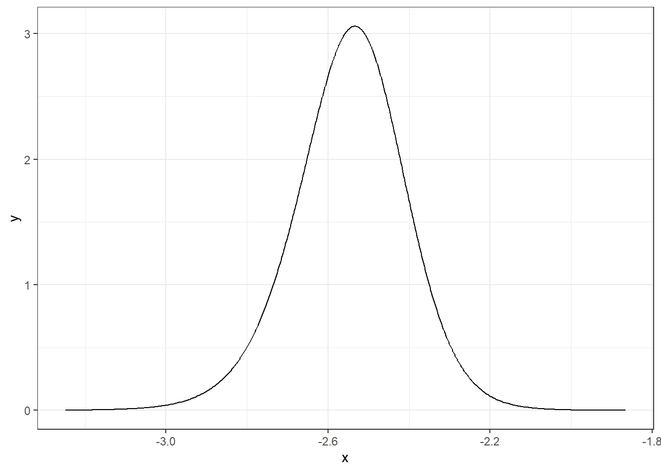

FIGURE 4.1: Posterior distribution of parameter \(\alpha\).

The quantile and the distribution functions are given by inla.qmarginal() and inla.pmarginal(), respectively. We can obtain the quantile 0.05 of \(\alpha\), and plot the probability that \(\alpha\) is lower than this quantile as follows:

quant <- inla.qmarginal(0.05, alpha)
quant

## [1] -2.785

inla.pmarginal(quant, alpha)

## [1] 0.05

A plot of the probability of \(\alpha\) being lower than the 0.05 quantile can be created as follows (Figure 4.2):

ggplot(data.frame(inla.smarginal(alpha)), aes(x, y)) +
  geom_line() +
  geom_area(data = subset(data.frame(inla.smarginal(alpha)),
                                     x < quant),
            fill = "black") +
  theme_bw()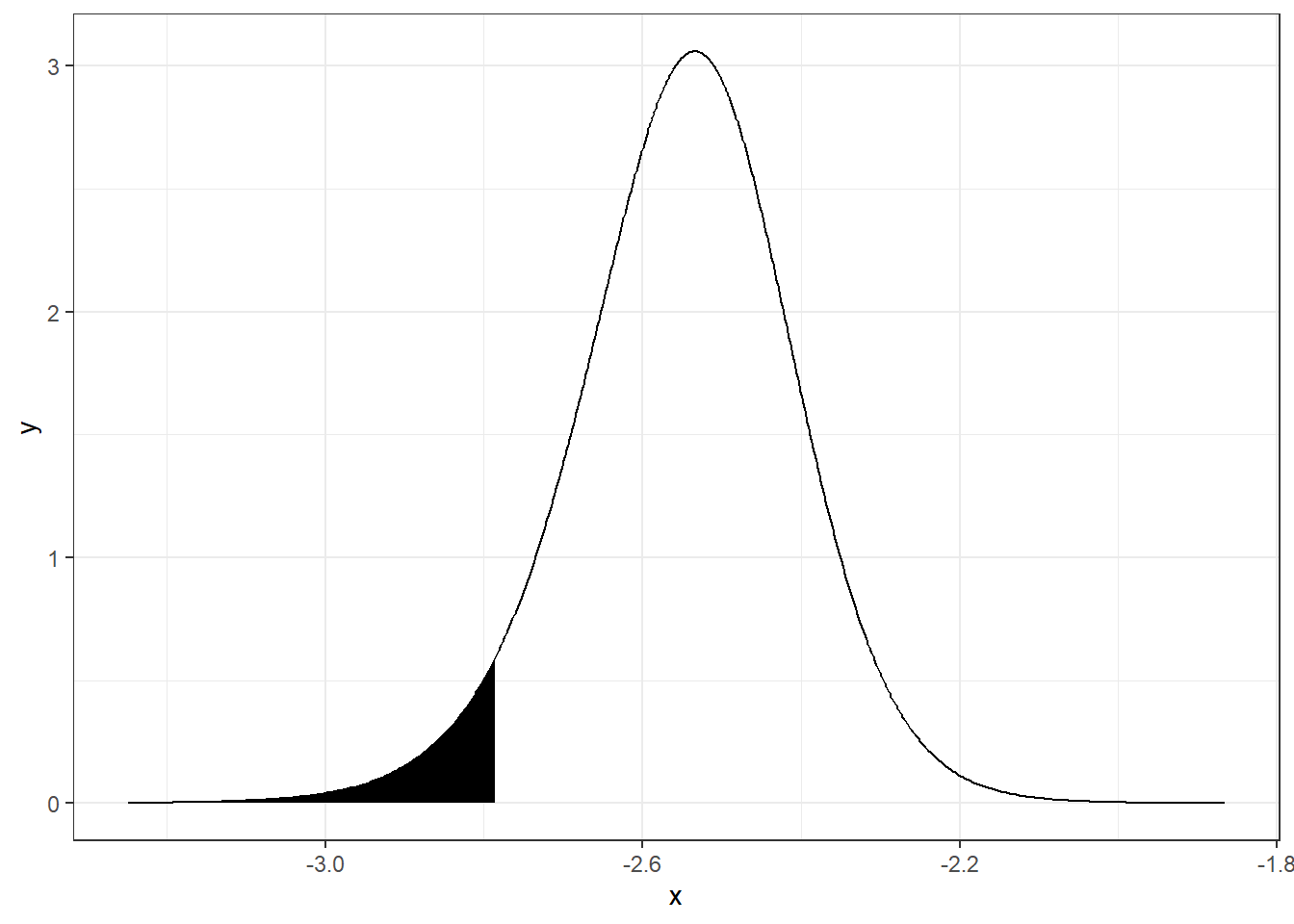

FIGURE 4.2: Probability of parameter \(\alpha\) being lower than the 0.05 quantile.

The function inla.dmarginal() computes the density at particular values. For example, the density at value -2.5 can be computed as follows (Figure 4.3):

inla.dmarginal(-2.5, alpha)

## [1] 2.943

ggplot(data.frame(inla.smarginal(alpha)), aes(x, y)) +
  geom_line() +
  geom_vline(xintercept = -2.5, linetype = "dashed") +
  theme_bw()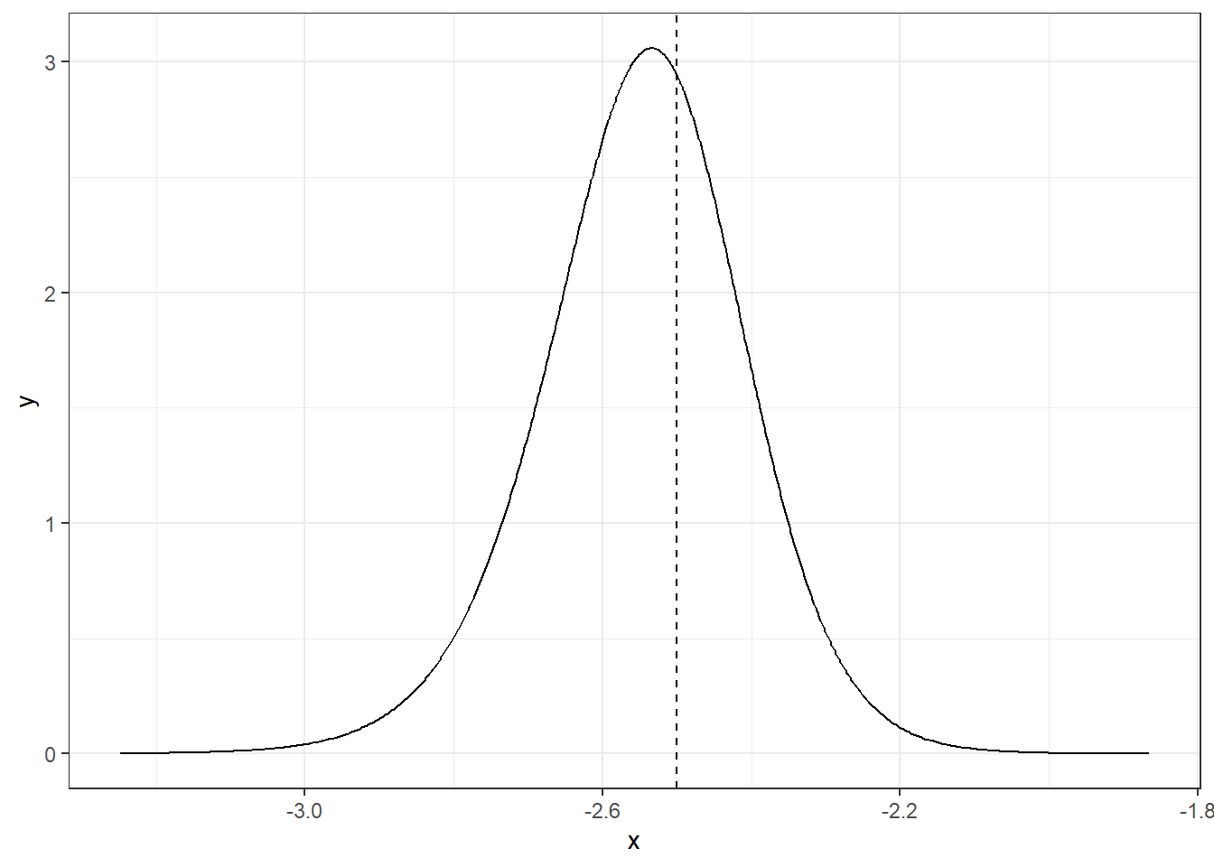

FIGURE 4.3: Posterior distribution of parameter \(\alpha\) at value -2.5.

If we wish to obtain a transformation of the marginal, we can use inla.tmarginal(). For example, if we wish to obtain the variance of the random effect \(u_i\), we can get the marginal of the precision \(\tau\) and then apply the inverse function.

marg.variance <- inla.tmarginal(function(x) 1/x,
res$marginals.hyperpar$"Precision for hospital")

A plot of the posterior of the variance of the random effect \(u_i\) is shown in Figure 4.4.

ggplot(data.frame(inla.smarginal(marg.variance)), aes(x, y)) +
  geom_line() +
  theme_bw()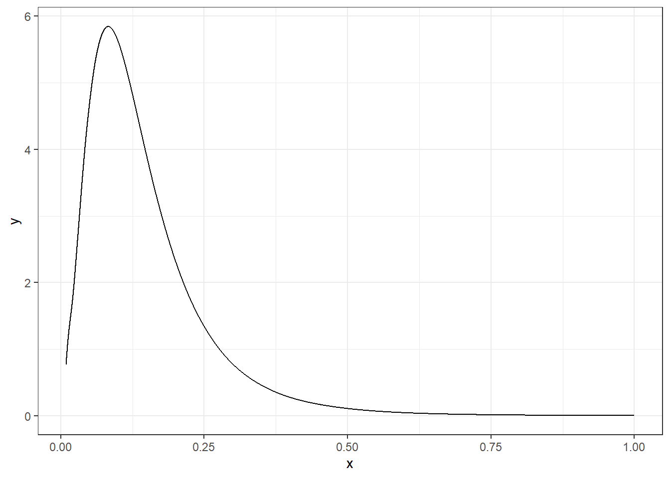

FIGURE 4.4: Posterior distribution of the variance of the random effect \(u_i\).

Now, if we wish to obtain the mean posterior of the variance, we can use inla.emarginal().

m <- inla.emarginal(function(x) x, marg.variance)
m

## [1] 0.1466

The standard deviation can be calculated using the expression \(Var[X] = E[X^2]- E[X]^2\).

mm <- inla.emarginal(function(x) x^2, marg.variance)
sqrt(mm - m^2)

## [1] 0.1044

Quantiles are calculated using the inla.qmarginal() function.

inla.qmarginal(c(0.025, 0.5, 0.975), marg.variance)

## [1] 0.02539 0.12065 0.42069

We can also use inla.zmarginal() to obtain summary statistics of the marginal.

inla.zmarginal(marg.variance)

## Mean            0.146626 
## Stdev           0.104365 
## Quantile  0.025 0.0253876 
## Quantile  0.25  0.075682 
## Quantile  0.5   0.120654 
## Quantile  0.75  0.187044 
## Quantile  0.975 0.420685

In this example, we wish to assess the performance of the hospitals by examining the mortality rates. res$marginals.fitted.values is a list that contains the posterior mortality rates of each of the hospitals. We can plot these posteriors by constructing a data frame marginals from the list res$marginals.fitted.values, and adding a column hospital denoting the hospital.

list_marginals <- res$marginals.fitted.values

marginals <- data.frame(do.call(rbind, list_marginals))
marginals$hospital <- rep(names(list_marginals),
                           times = sapply(list_marginals, nrow))

Then, we can plot marginals with ggplot() using facet_wrap() to make one plot per hospital. Figure 4.5 shows that hospitals 2, 8 and 11 have the highest mortality rates and, therefore, have poorer performance than the rest.

library(ggplot2)
ggplot(marginals, aes(x = x, y = y)) + geom_line() +
  facet_wrap(~ hospital) +
  labs(x = "", y = "Density") +
  geom_vline(xintercept = 0.1, col = "gray") +
  theme_bw()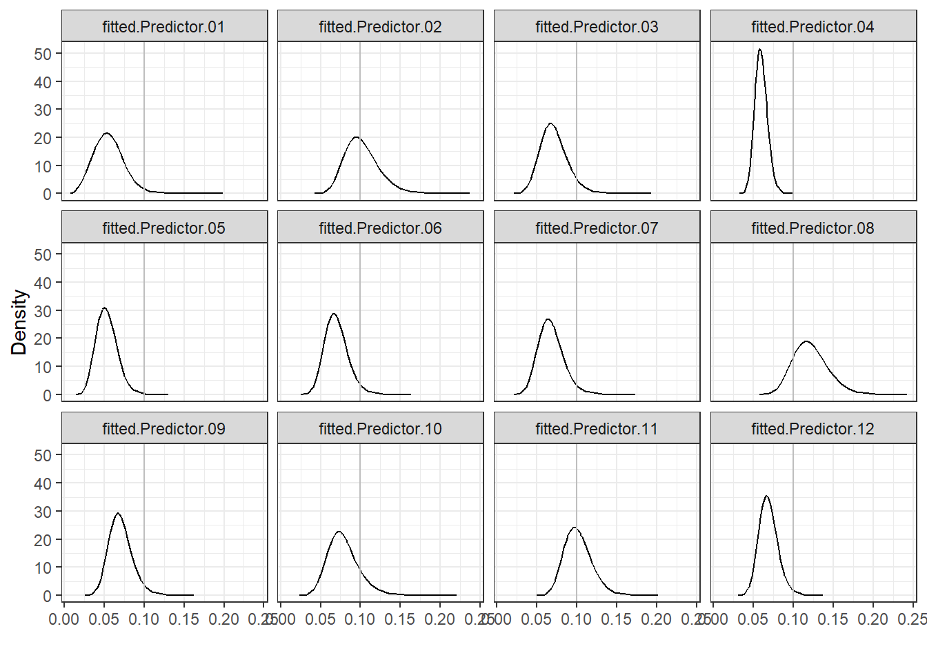

FIGURE 4.5: Posterior distributions of mortality rates of each hospital.

We can also compute the probabilities that mortality rates are greater than a given threshold value. These probabilities are called exceedance probabilities and are expressed as \(P(p_i > c)\), where \(p_i\) represents the mortality rate of hospital \(i\) and \(c\) is the threshold value. For example, we can calculate the probability that the mortality rate of hospital 1, \(p_1\), is higher than \(c\) using \(P(p_1 > c) = 1 - P(p_1 \leq c)\). In R-INLA, \(P(p_1 \leq c)\) can be calculated with the inla.pmarginal() function passing as arguments the marginal distribution of \(p_1\) and the threshold value \(c\). The marginals of the mortality rates are in the list res$marginals.fitted.values, and the marginal corresponding to the first hospital is res$marginals.fitted.values[[1]]. We can choose \(c\) equal to 0.1 and calculate \(P(p_1 > 0.1)\) as follows:

marg <- res$marginals.fitted.values[[1]]
1 - inla.pmarginal(q = 0.1, marginal = marg)

## [1] 0.01734

We can calculate the probabilities that mortality rates are greater than 0.1 for all hospitals using the sapply() function passing as arguments the list with all the marginals (res$marginals.fitted.values), and the function to calculate the exceedance probabilities (1- inla.pmarginal()). sapply() returns a vector of the same length as the list res$marginals.fitted.values with values equal to the result of applying the function 1- inla.pmarginal() to each of the elements of the list of marginals.

sapply(res$marginals.fitted.values,
FUN = function(marg){1-inla.pmarginal(q = 0.1, marginal = marg)})

## fitted.Predictor.01 fitted.Predictor.02 
##           1.734e-02           4.843e-01 
## fitted.Predictor.03 fitted.Predictor.04 
##           5.722e-02           3.952e-06 
## fitted.Predictor.05 fitted.Predictor.06 
##           1.225e-03           2.952e-02 
## fitted.Predictor.07 fitted.Predictor.08 
##           2.966e-02           8.374e-01 
## fitted.Predictor.09 fitted.Predictor.10 
##           3.043e-02           1.269e-01 
## fitted.Predictor.11 fitted.Predictor.12 
##           4.916e-01           9.177e-03

These exceedance probabilities indicate that the probability that mortality rate exceeds 0.1 is highest for hospital 8 (probability equal to 0.83), and lowest for hospital 4 (probability equal to \(4.36 \times 10^{-6}\)).

Finally, it is also possible to generate samples from an approximated posterior of a fitted model using the inla.posterior.sample() function passing as arguments the number of samples to be generated, and the result of an inla() call that needs to have been created using the option control.compute = list(config = TRUE).

4.5 Control variables to compute approximations

The inla() function has an argument called control.inla that permits to specify a list of variables to obtain more accurate approximations or reduce the computational time. The approximations of the posterior marginals are computed using numerical integration. Different strategies can be considered to choose the integration points \(\{ \boldsymbol{\theta_k} \}\) by specifying the argument int.strategy. One possibility is to use a grid around the mode of \(\tilde \pi(\boldsymbol{\theta}|\boldsymbol{y})\). This is the most costly option and can be obtained with the command control.inla = list(int.strategy = "grid"). The complete composite design is less costly when the dimension of the hyperparameters is relatively large and it is specified as control.inla = list(int.strategy = "ccd"). An alternative strategy is to use only one integration point equal to the posterior mode of the hyperparameters. This corresponds to an empirical Bayes approach and can be obtained with the command control.inla = list(int.strategy = "eb"). The default option is control.inla = list(int.strategy = "auto") which corresponds to "grid" if \(|\boldsymbol{\theta}| \leq 2\), and "ccd" otherwise. Moreover, the inla.hyperpar() function can be used with the result object of an inla() call to improve the estimates of the posterior marginals of the hyperparameters using the grid integration strategy.

The argument strategy is used to specify the method to obtain the approximations for the posterior marginals for \(x_i\)’s conditioned on selected values of \(\boldsymbol{\theta_k}\), \(\tilde \pi(x_i|\boldsymbol{\theta_k},\boldsymbol{y})\). The possible options are strategy = "gaussian", strategy = "laplace", strategy = "simplified.laplace", and strategy = "adaptative". The "adaptative" option chooses between the "gaussian" and the "simplified.laplace" options. The default option is "simplified.laplace" and this represents a compromise between accuracy and computational cost.