10 Spatio-temporal modeling of geostatistical data. Air pollution in Spain
In this chapter we show how to fit a spatio-temporal model to predict fine particulate air pollution levels (PM\(_{2.5}\)) in Spain over the years 2015 to 2017 using the stochastic partial differential equation (SPDE) approach and the R-INLA package (Havard Rue, Lindgren, and Teixeira Krainski 2024). PM\(_{2.5}\) are a mixture of solid particles and liquid droplets less than 2.5 micrometers in diameter that are floating in the air. These particles come from various sources including motor vehicles, power plants and forest fires. Monitoring of PM\(_{2.5}\) is important since these particles harm the environment and can cause serious health conditions including respiratory and cardiovascular diseases and premature death.
We retrieve air pollution values measured at several monitoring stations in Spain over the years 2015 to 2017 from the European Environment Agency, and obtain a map of Spain using the raster package (Hijmans 2023). Then we fit a spatio-temporal model to predict air pollution at locations where measurements are not available and construct high-resolution maps of air pollution for each year. We also show how to visualize the model predictions and 95% credible intervals denoting uncertainty using several maps constructed with the ggplot2 package (Wickham et al. 2024).
10.1 Map
We obtain the map of Spain using the getData() function of the raster package (Hijmans 2023).
We set name equal to GADM which is the database of global administrative boundaries, country equal to Spain, and level equal to 0 which corresponds to the level of administrative subdivision country (Figure 10.1).
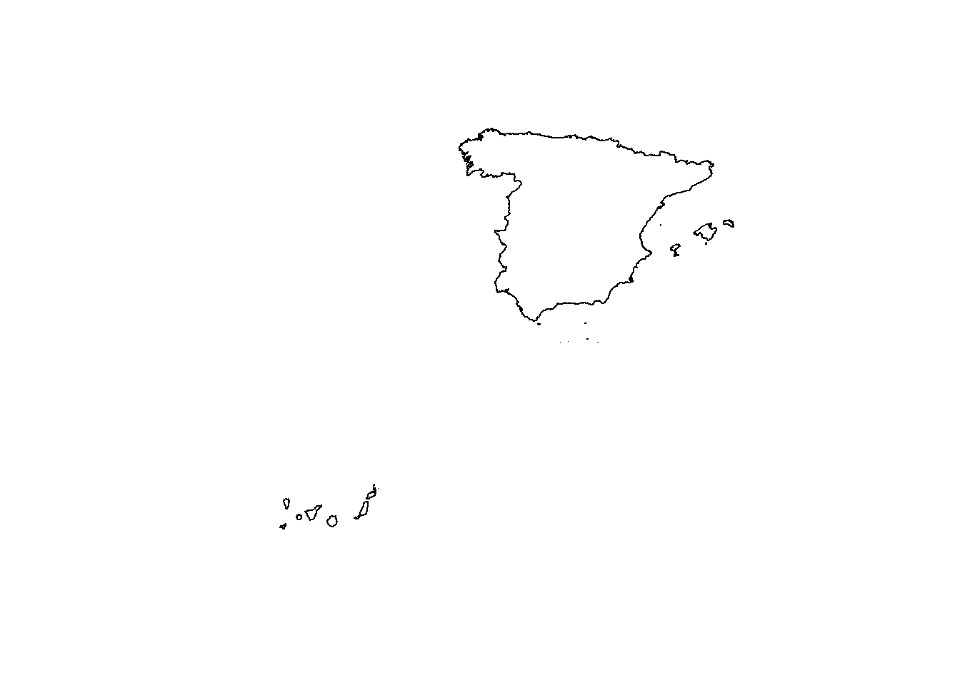
FIGURE 10.1: Map of Spain.
We are only interested in predicting air pollution in the main territory of Spain, and therefore we remove the islands from the map. We can do this by keeping the polygon of the map that has the largest area using the packages sf and dplyr. First, we convert m which is a SpatialPolygonsDataFrame object to an sf object. Then we calculate the areas of the polygons of the object, and keep the polygon with the largest area.
library(sf)
library(dplyr)

m <- m %>%
  st_as_sf() %>%
  st_cast("POLYGON") %>%
  mutate(area = st_area(.)) %>%
  arrange(desc(area)) %>%
  slice(1)
The final map can be shown with the ggplot() function of ggplot2 (Figure 10.2).
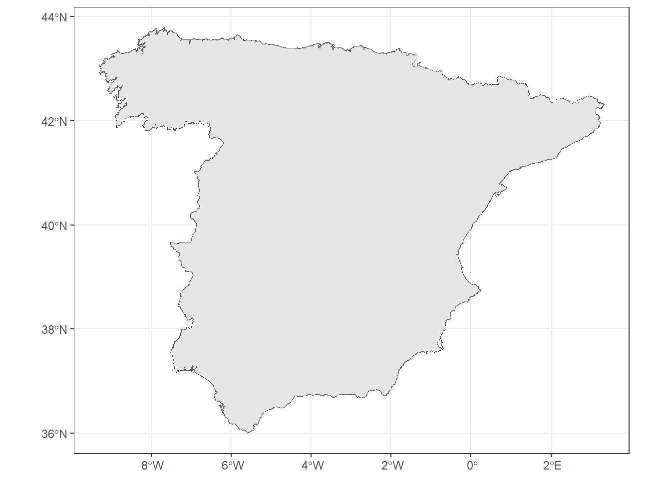
FIGURE 10.2: Map of Spain without islands.
The object map has a geographic coordinate system with longitude and latitude values.
We transform map to an object with UTM projection because we wish to work with meters.
To do this, we use the st_transform() function specifying the ESPG code of Spain which is code 25830 and corresponds to UTM zone 30 North.
We plot map with ggplot() and use coord_sf(datum = st_crs(m)) to show the graticule and coordinates corresponding to the map projection
(Figure 10.3).
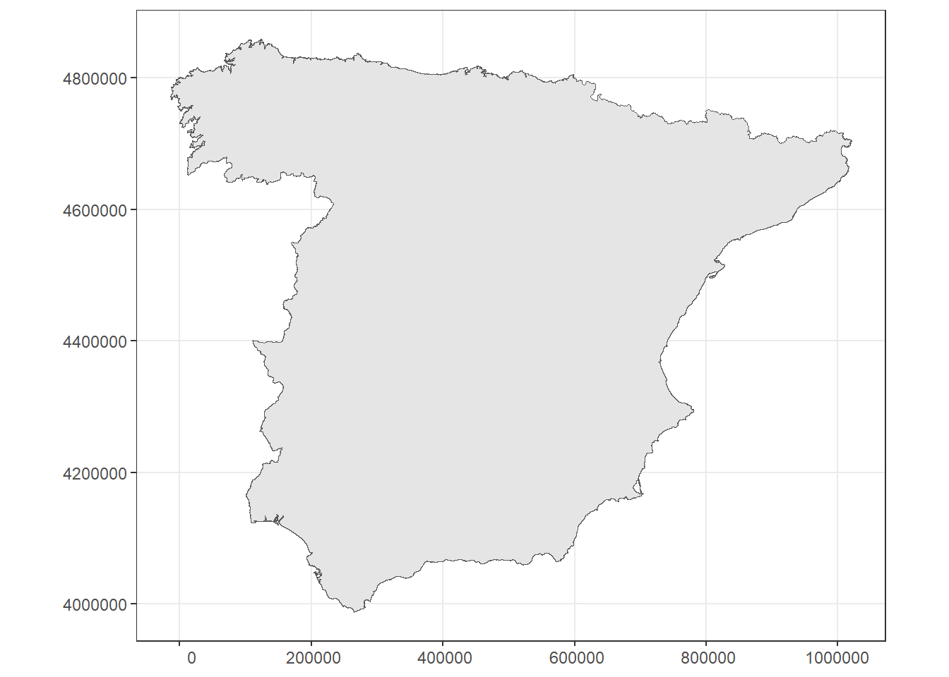
FIGURE 10.3: Map of Spain without islands and with UTM projection.
10.2 Data
Air pollution measurements recorded at monitoring stations in Spain and other European countries can be obtained from the European Environment Agency. Here we use data of the annual averages of fine particulate matter (PM\(_{2.5}\)) levels recorded at monitoring stations in Spain in years 2015, 2016 and 2017.
A CSV file called dataPM25.csv that contains these data can be downloaded from the book webpage.
We save this file in our computer and then read it with the read.csv() function.
We keep only the variables of the data that indicate year, id of monitoring station, longitude, latitude and PM\(_{2.5}\) values, and assign new names to these columns.
d <- read.csv("dataPM25.csv")
d <- d[, c(
  "ReportingYear", "StationLocalId",
  "SamplingPoint_Longitude",
  "SamplingPoint_Latitude",
  "AQValue"
)]
names(d) <- c("year", "id", "long", "lat", "value")
Now we project the data which uses geographical coordinates to UTM projection.
First, we create an sf object called p with the longitude and latitude values of the monitoring stations, and set the CRS of p to EPSG 4326 which corresponds to geographical coordinates. Then we use st_transform() to project the data to EPSG code 25830. Finally, we substitute the geographical coordinates of the data d by the UTM coordinates.
p <- st_as_sf(data.frame(long = d$long, lat = d$lat),
              coords = c("long", "lat"))
st_crs(p) <- st_crs(4326)
p <- p %>% st_transform(25830)
d[, c("x", "y")] <- st_coordinates(p)
Now we keep only the observations corresponding to monitoring stations located within the main territory of Spain and remove the observations from the islands.
We do this by finding the indices of the locations that intersect with the map with st_intersects(),
and keeping the rows of d that contain the locations within the map.
ind <- st_intersects(m, p)
d <- d[ind[[1]], ]
A map showing the locations of the monitoring stations in the main territory of Spain is shown in Figure 10.4.
ggplot(m) + geom_sf() + coord_sf(datum = st_crs(m)) +
  geom_point(data = d, aes(x = x, y = y)) + theme_bw()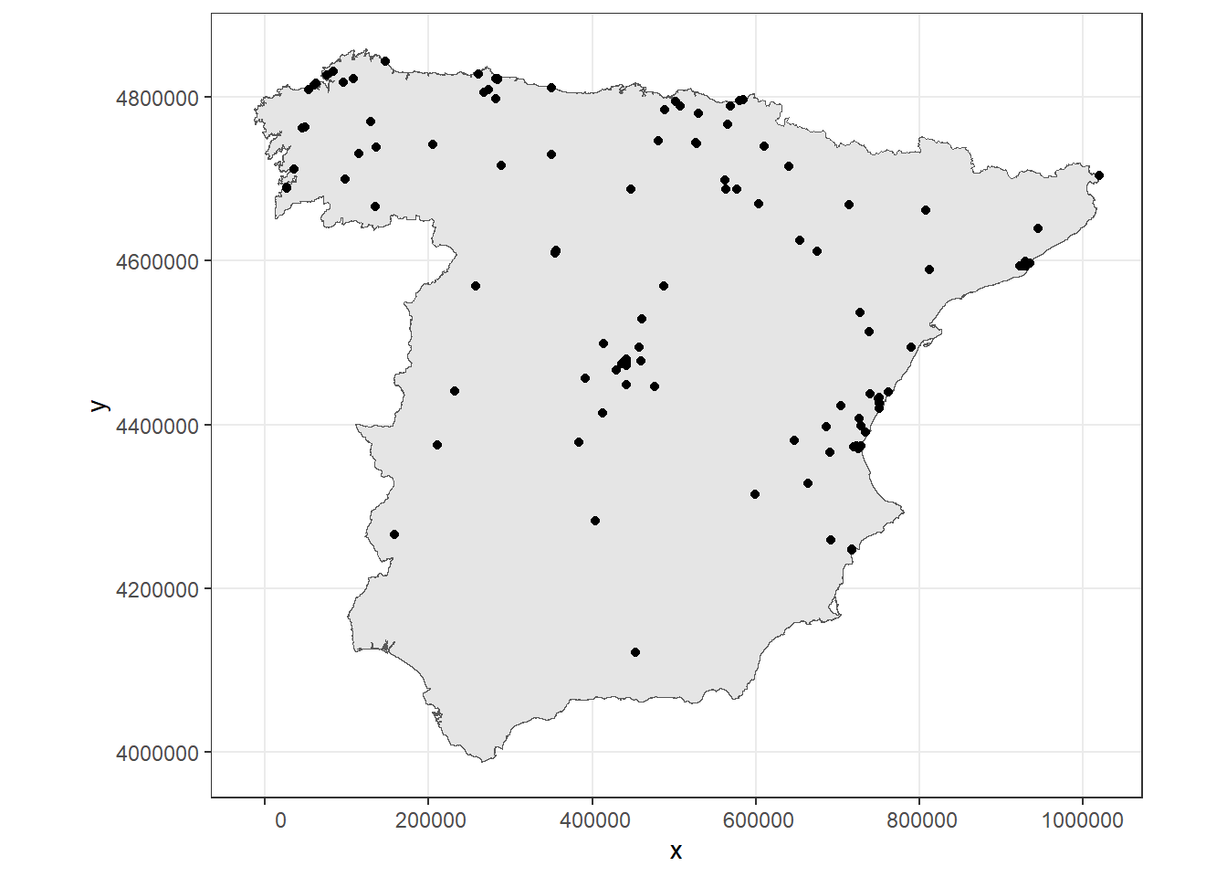
FIGURE 10.4: Monitoring stations of PM\(_{2.5}\).
We can visualize the PM\(_{2.5}\) values by means of several plots.
For example, we can make histograms of the values of each year using geom_histogram() and facet_wrap()
(Figure 10.5).
ggplot(d) +
  geom_histogram(mapping = aes(x = value)) +
  facet_wrap(~year, ncol = 1) +
  theme_bw()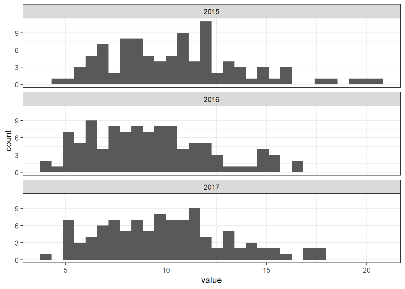
FIGURE 10.5: Histograms of PM\(_{2.5}\) values for each year.
We can also make maps of the PM\(_{2.5}\) values in each monitoring station over time using geom_point().
We use coord_sf(datum = NA) to remove the map graticule and coordinates,
facet_wrap() to create maps for each year, and scale_color_viridis() to use the viridis color scale
(Figure 10.6).
library(viridis)

ggplot(m) + geom_sf() + coord_sf(datum = NA) +
  geom_point(
    data = d, aes(x = x, y = y, color = value),
    size = 2
  ) +
  labs(x = "", y = "") +
  scale_color_viridis() +
  facet_wrap(~year) +
  theme_bw()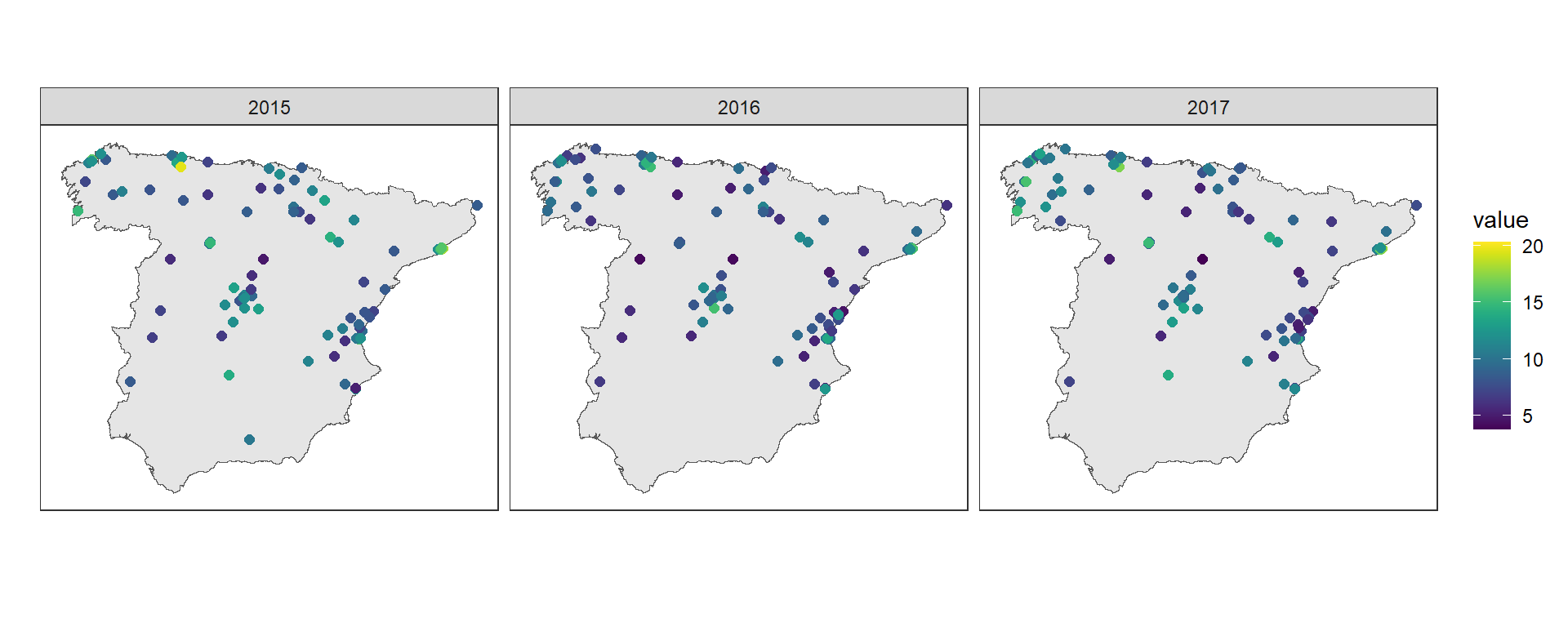
FIGURE 10.6: PM\(_{2.5}\) values recorded in the monitoring stations.
Next, we produce a time plot showing PM\(_{2.5}\) values over time in each monitoring station using geom_line().
We use scale_y_continuous() with breaks set to the years for the y axis, and
decide to remove the legend using theme(legend.position = "none") since it occupies a large part of the plot
(Figure 10.7).
ggplot(d, aes(x = year, y = value, group = id, color = id)) +
  geom_line() +
  geom_point(size = 2) +
  scale_x_continuous(breaks = c(2015, 2016, 2017)) +
  theme_bw() + theme(legend.position = "none")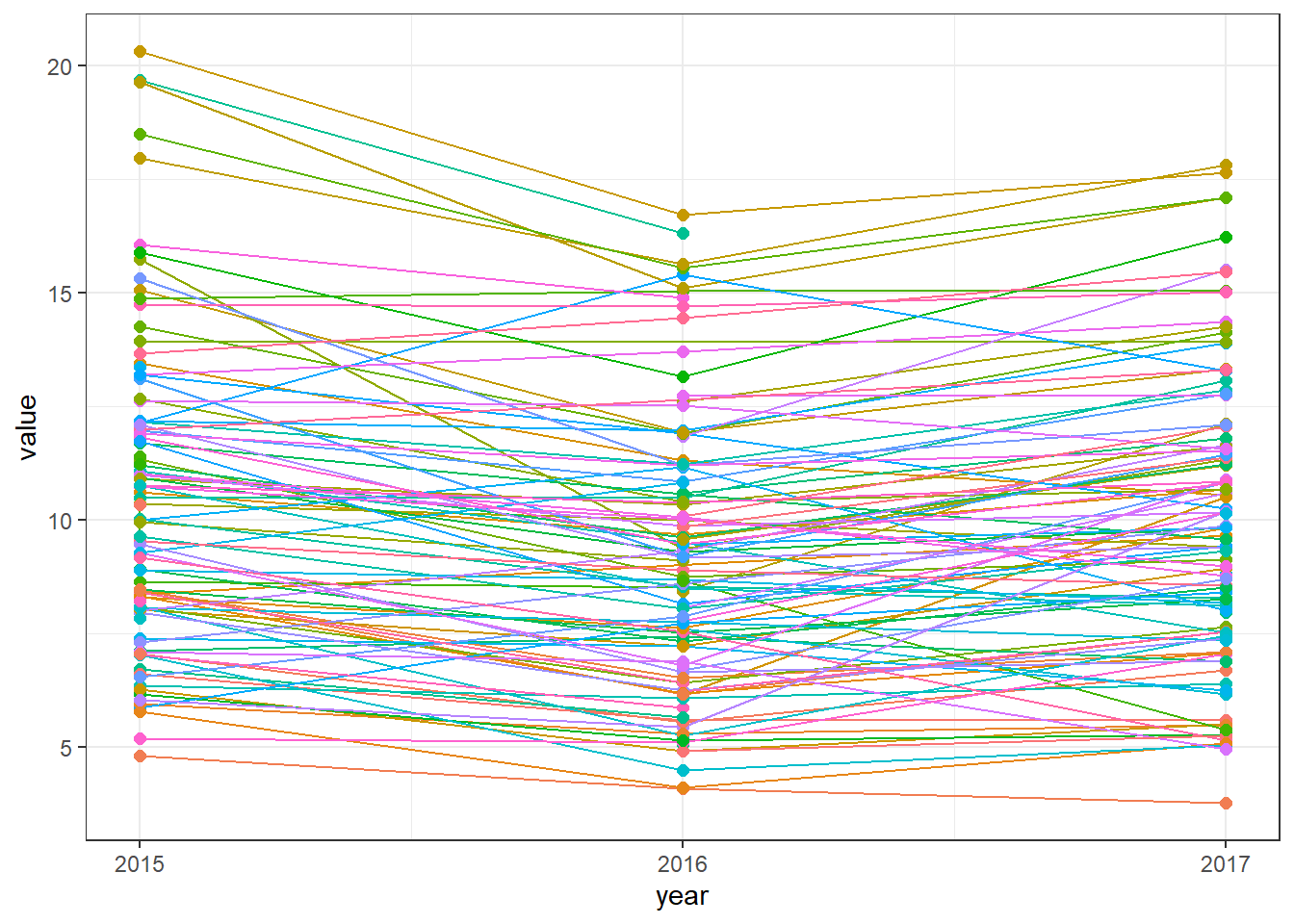
FIGURE 10.7: Time plot of PM\(_{2.5}\) values for each of the monitoring stations.
10.3 Modeling
In this section we show how to specify a spatio-temporal model to predict PM\(_{2.5}\) and the steps required to fit the model using R-INLA.
10.3.1 Model
Let \(Y_{it}\) be the PM\(_{2.5}\) values measured at locations \(i=1,\ldots,I\) and times \(t=1,2,3.\) The model assumes
\[Y_{it} \sim N(\mu_{it} , \sigma_e^2),\]
\[\mu_{it} = \beta_0 + \xi(\boldsymbol{x}_i, t),\]
where \(\beta_0\) is the intercept, \(\sigma_e^2\) is the variance of the measurement error, and \(\xi(\boldsymbol{x}_i, t)\) is a spatio-temporal random effect at location \(\boldsymbol{x}_i\) and time \(t\). We define \(\sigma_e^2\) as a zero-mean Gaussian process both temporal and spatially uncorrelated. \(\xi(\boldsymbol{x}_i, t)\) is a random effect that changes in time with first order autoregressive dynamics and spatially correlated innovations. Specifically,
\[\xi(\boldsymbol{x}_i, t) = a \xi(\boldsymbol{x}_i, t-1) + w(\boldsymbol{x}_i, t),\] where \(|a|<1\) and \(\xi(\boldsymbol{x}_i, 1)\) follows a stationary distribution of a first-order autoregressive process, namely, \(N(0, \sigma^2_w/(1-a^2))\). Each \(w(\boldsymbol{x}_i, t)\) follows a zero-mean Gaussian distribution temporally independent but spatially dependent at each time with Matérn covariance function.
Thus, this model includes an intercept and a spatio-temporal random effect that changes in time with first order autoregressive dynamics and spatially correlated innovations, but does not include covariates. In real applications models can include covariates related to air pollution such as temperature, precipitation or distance to roads, and this will improve predictive performance.
10.3.2 Mesh construction
To fit the model with the SPDE approach, we need to construct a triangulated mesh on top of which the GMRF representation is built. The mesh needs to cover the region of study and also an outer extension to avoid boundary effects by which the variance is increased near the boundary. In this example, we decide to use the mesh specified below so the model can be run in a reasonable time but a finer mesh could be considered in real applications.
We create the mesh using the inla.mesh.2d() function and the following arguments.
We set loc equal to the matrix with the coordinates (coo) so they are used as initial mesh vertices.
The boundary of the mesh is equal to a polygon containing the map locations constructed with the inla.nonconvex.hull() function.
We set the maximum allowed triangle edge lengths in the region and in the extension with max.edge = c(100000, 200000). This permits to use small triangles within the region, and larger triangles in the extension where there is no data and we do not want to waste computational resources.
We specify the minimum allowed distance between points with cutoff = 1000 to avoid building many small triangles where we have some very close points.
Further details about the arguments inla.mesh.2d() and inla.nonconvex.hull() can be seen in the help files of the R-INLA package.
library(INLA)

coo <- cbind(d$x, d$y)
bnd <- inla.nonconvex.hull(st_coordinates(m)[, 1:2])
mesh <- inla.mesh.2d(
  loc = coo, boundary = bnd,
  max.edge = c(100000, 200000), cutoff = 1000
)
The number of vertices of the mesh is given by mesh$n and we can plot the mesh with plot(mesh) (Figure 10.8).
mesh$n## [1] 729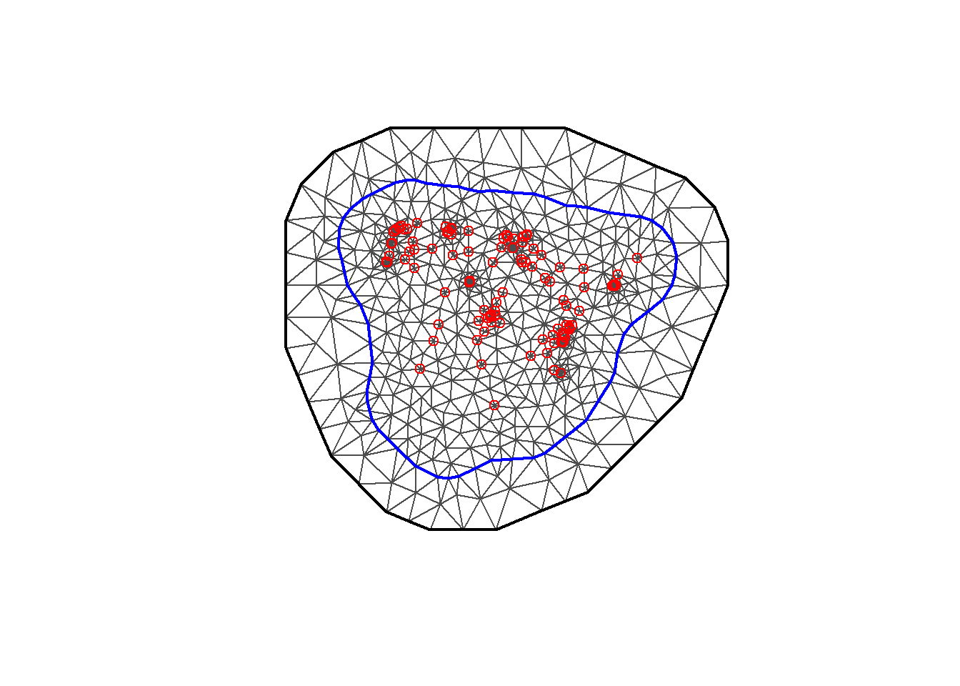
FIGURE 10.8: Triangulated mesh used to build the SPDE model.
10.3.3 Building the SPDE model on the mesh
Now we use the inla.spde2.pcmatern() function to build the SPDE model and specify
Penalised Complexity (PC) priors for the parameters of the Matérn field
(Fuglstad et al. 2019).
The first two arguments of inla.spde2.pcmatern() are
mesh which denotes mesh object,
and alpha which is related to the smoothness of the process.
In this example, we are dealing with spatial data (\(d=2\)), and we fix the smoothness parameter \(\nu\) equal to one.
Thus, \(\alpha=\nu+d/2 = 2\).
We also set constr = TRUE to impose an integrate-to-zero constraint.
PC priors for the parameters range and marginal standard deviation of the Matérn field are specified by setting the values \(v_r\), \(p_r\), \(v_s\) and \(p_s\) in the relations
\(P(range < v_r) = p_r\) and
\(P(\sigma > v_s) = p_s\).
The range of the process is the distance such that the correlation between values is close to 0.1.
In this example, we decide to use a prior \(P(range < 10000) = 0.01\) which means that the probability that the range is less than 10 km is very small.
The parameter \(\sigma\) denotes the variability of the data.
We specify the prior for this parameter as \(P(\sigma > 3) = 0.01\).
These PC priors are specified in the arguments prior.range and prior.sigma of the inla.spde2.pcmatern() function as follows:
spde <- inla.spde2.pcmatern(
  mesh = mesh, alpha = 2, constr = TRUE,
  prior.range = c(10000, 0.01), # P(range < 10000) = 0.01
  prior.sigma = c(3, 0.01) # P(sigma > 3) = 0.01
)
10.3.4 Index set
Now we contruct the index set for the latent spatio-temporal Gaussian model using inla.spde.make.index(). We need to specify the name (s), the number of vertices in the SPDE model (spde$n.spde), and the number of times (timen).
Note here that the index set does not depend on the locations of the data.
timesn <- length(unique(d$year))
indexs <- inla.spde.make.index("s",
  n.spde = spde$n.spde,
  n.group = timesn
)
lengths(indexs)
## s s.group s.repl
## 2187 2187 2187The index set created (indexs) is a list containing three elements:
-
s: indices of the SPDE vertices repeated the number of times, -
s.group: indices of the times repeated the number of mesh vertices, -
s.repl: vector of 1s with length given by the number of mesh vertices times the number of times (spde$n.spde*timesn).
10.3.5 Projection matrix
Now we build a projection matrix \(A\) that projects the spatio-temporal continuous Gaussian random field from the observations to the mesh nodes.
The projection matrix can be built with the inla.spde.make.A() function by providing the arguments mesh,
the coordinates (loc), and the time indices (group) of the observations.
group is a vector of length equal to the number of observations and elements equal to 1, 2, or 3 denoting, respectively, years 2015, 2016 and 2017.
group <- d$year - min(d$year) + 1
A <- inla.spde.make.A(mesh = mesh, loc = coo, group = group)
10.3.6 Prediction data
Now we construct the data with the locations and times where we want to make predictions.
We predict at locations within the main territory of Spain region and in years 2015, 2016 and 2017.
First, we create a grid of \(50 \times 50\) locations by using expand.grid() and combining vectors x and y which contain the coordinates in the range of the observation locations (Figure 10.9). We call the data for prediction dp.
bb <- st_bbox(m)
x <- seq(bb$xmin - 1, bb$xmax + 1, length.out = 50)
y <- seq(bb$ymin - 1, bb$ymax + 1, length.out = 50)
dp <- as.matrix(expand.grid(x, y))
plot(dp, asp = 1)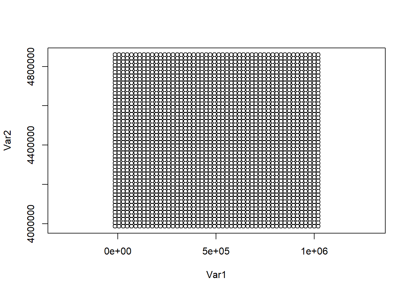
FIGURE 10.9: Grid locations for prediction.
Then, we keep only the locations that lie within the map of Spain (Figure 10.10).
p <- st_as_sf(data.frame(x = dp[, 1], y = dp[, 2]),
  coords = c("x", "y")
)
st_crs(p) <- st_crs(25830)
ind <- st_intersects(m, p)
dp <- dp[ind[[1]], ]
plot(dp, asp = 1)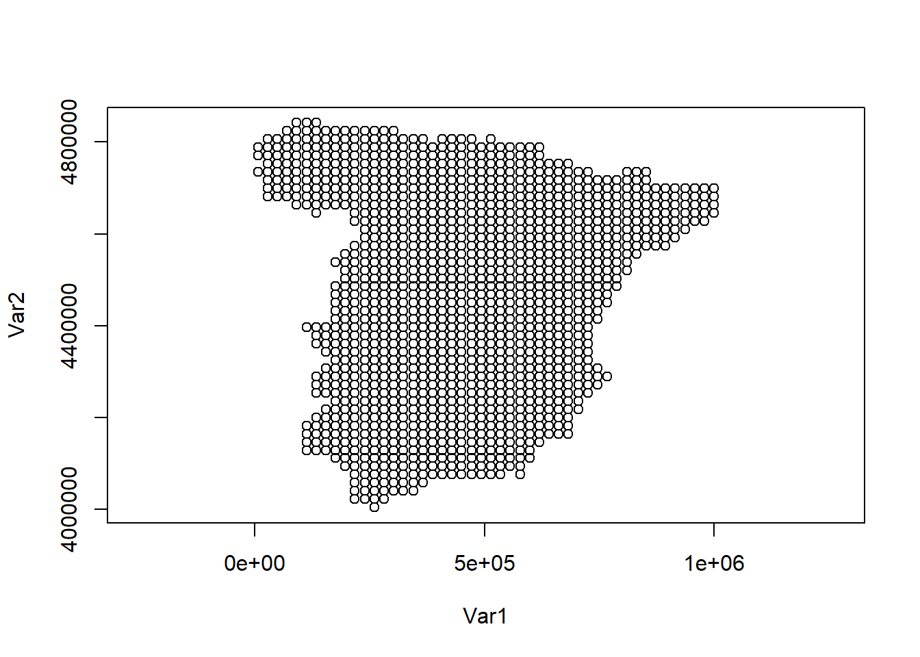
FIGURE 10.10: Locations for prediction in Spain.
Now we construct the data that includes the coordinates and the three times by repeating dp three times and adding a column denoting the times.
Here time 1 is 2015, time 2 is 2016, and time 3 is 2017.
##        Var1    Var2
## [1,] 260559 4004853 1
## [2,] 218306 4022657 1
## [3,] 239432 4022657 1
## [4,] 260559 4022657 1
## [5,] 281685 4022657 1
## [6,] 218306 4040460 1
Finally, we also construct the matrix Ap that projects the spatially continuous Gaussian random field from the prediction locations to the mesh nodes.
Prediction locations are in coop and time indices are in groupp.
coop <- dp[, 1:2]
groupp <- dp[, 3]
Ap <- inla.spde.make.A(mesh = mesh, loc = coop, group = groupp)
10.3.7 Stack with data for estimation and prediction
Now we construct the stacks for estimation (stk.e) and prediction (stk.p) using inla.stack()
and the following arguments:
-
tag: string for identifying the data, -
data: list of data vectors, -
A: list of projection matrices, -
effects: list with fixed and random effects.
Then we put both stacks together in a full stack called stk.full.
stk.e <- inla.stack(
  tag = "est",
  data = list(y = d$value),
  A = list(1, A),
  effects = list(data.frame(b0 = rep(1, nrow(d))), s = indexs)
)

stk.p <- inla.stack(
  tag = "pred",
  data = list(y = NA),
  A = list(1, Ap),
  effects = list(data.frame(b0 = rep(1, nrow(dp))), s = indexs)
)

stk.full <- inla.stack(stk.e, stk.p)
10.3.8 Model formula
Now we define the formula that we use to fit the model.
In the formula we remove the intercept (adding 0) and add it as a covariate term (adding b0).
The SPDE model is specified with f() adding the name s, the model spde, the group given by the indices s.group of indexs, and the control group with list(model = "ar1", hyper = rprior).
By using group = s.group we specify that in each of the years, the spatial locations are linked by the SPDE model.
control.group = list(model = "ar1", hyper = rprior) specifes that across time, the process evolves according to an AR(1) process
where the prior for the autocorrelation parameter \(a\) is given by rprior.
We define rprior with the prior "pccor1" which is a PC prior for the autocorrelation parameter \(a\) where \(a = 1\) is the base model.
Here we assume \(P(a > 0) = 0.9\).
The formula is defined as
10.3.9 inla() call
Finally, we call inla() providing the formula, data, and options. In control.predictor we specify the projection matrix and compute = TRUE to obtain the predictions.
res <- inla(formula,
  data = inla.stack.data(stk.full),
  control.predictor = list(
    compute = TRUE,
    A = inla.stack.A(stk.full)
  )
)
10.3.10 Results
We can inspect the results by typing summary(res). This shows the parameter estimates of the fixed and random effects.
summary(res)## Time used:
## Pre = 2.77, Running = 10.3, Post = 0.243, Total = 13.3
## Fixed effects:
## mean sd 0.025quant 0.5quant 0.975quant mode
## b0 8.543 0.295 7.966 8.542 9.126 8.542
## kld
## b0 0
##
## Random effects:
## Name Model
## s SPDE2 model
##
## Model hyperparameters:
## mean
## Precision for the Gaussian observations 8.96e-01
## Range for s 1.80e+04
## Stdev for s 5.20e+00
## GroupRho for s 9.66e-01
## sd
## Precision for the Gaussian observations 0.177
## Range for s 1828.799
## Stdev for s 0.412
## GroupRho for s 0.013
## 0.025quant
## Precision for the Gaussian observations 5.94e-01
## Range for s 1.46e+04
## Stdev for s 4.44e+00
## GroupRho for s 9.34e-01
## 0.5quant
## Precision for the Gaussian observations 8.81e-01
## Range for s 1.79e+04
## Stdev for s 5.19e+00
## GroupRho for s 9.68e-01
## 0.975quant
## Precision for the Gaussian observations 1.29e+00
## Range for s 2.18e+04
## Stdev for s 6.06e+00
## GroupRho for s 9.86e-01
## mode
## Precision for the Gaussian observations 8.55e-01
## Range for s 1.77e+04
## Stdev for s 5.15e+00
## GroupRho for s 9.72e-01
##
## Marginal log-Likelihood: -677.44
## is computed
## Posterior summaries for the linear predictor and the fitted values are computed
## (Posterior marginals needs also 'control.compute=list(return.marginals.predictor=TRUE)')We can create plots of the posterior distributions of the intercept, the precision of the measurement error, and the standard deviation, range and autocorrelation parameters of the spatio-temporal random effect.
We do this by constructing a list called list_marginals with the posterior distributions of each parameter. Then we construct a data frame marginals from this list, and add a column parameter with the name of the parameter of each distribution.
list_marginals <- list(
"b0" = res$marginals.fixed$b0,
"precision Gaussian obs" =
res$marginals.hyperpar$"Precision for the Gaussian observations",
"range" = res$marginals.hyperpar$"Range for s",
"stdev" = res$marginals.hyperpar$"Stdev for s",
"rho" = res$marginals.hyperpar$"GroupRho for s"
)


marginals <- data.frame(do.call(rbind, list_marginals))
marginals$parameter <- rep(names(list_marginals),
  times = sapply(list_marginals, nrow)
)
Finally, we plot marginals with ggplot() using facet_wrap() to make one plot per parameter
(Figure 10.11).
library(ggplot2)
ggplot(marginals, aes(x = x, y = y)) + geom_line() +
  facet_wrap(~parameter, scales = "free") +
  labs(x = "", y = "Density") + theme_bw()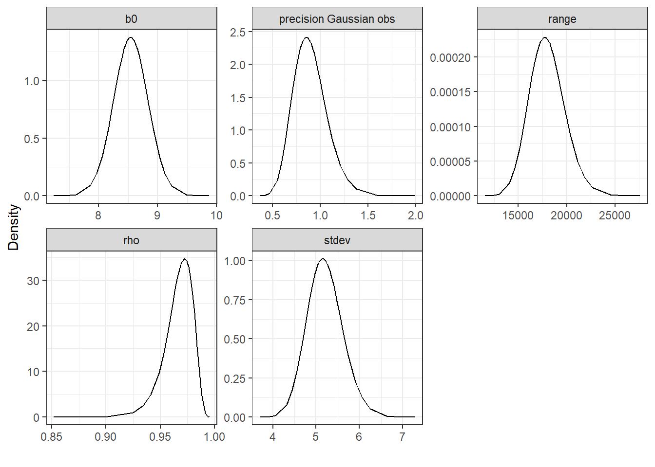
FIGURE 10.11: Posterior distributions of the model parameters.
10.4 Mapping air pollution predictions
We make maps of the predicted PM\(_{2.5}\) levels in Spain for years 2015, 2016 and 2017.
To retrieve the predictions obtained from the model, we use inla.stack.index() to get the indices of stk.full that correspond to tag = "pred".
index <- inla.stack.index(stack = stk.full, tag = "pred")$dataWe can obtain the mean predictions and lower and upper limits of the 95% credible intervals from the data frame res$summary.fitted.values.
We need to specify the rows of res$summary.fitted.values that correspond to the predictions (index) and the columns "mean", "0.025quant" and "0.975quant".
We assign each of the vectors to the data frame dp that contains the locations and times of the predictions.
dp <- data.frame(dp)
names(dp) <- c("x", "y", "time")

dp$pred_mean <- res$summary.fitted.values[index, "mean"]
dp$pred_ll <- res$summary.fitted.values[index, "0.025quant"]
dp$pred_ul <- res$summary.fitted.values[index, "0.975quant"]
To make the maps, we first
melt dp into a data frame dpm suitable for plotting.
We use the function melt from the reshape2 package. We specify the id variables are c("x", "y", "time") and the measured variables are c("pred_mean", "pred_ll", "pred_ul").
library(reshape2)
dpm <- melt(dp,
  id.vars = c("x", "y", "time"),
  measure.vars = c("pred_mean", "pred_ll", "pred_ul")
)
head(dpm)
## x y time variable value
## 1 260559 4004853 1 pred_mean 8.541
## 2 218306 4022657 1 pred_mean 8.541
## 3 239432 4022657 1 pred_mean 8.541
## 4 260559 4022657 1 pred_mean 8.541
## 5 281685 4022657 1 pred_mean 8.541
## 6 218306 4040460 1 pred_mean 8.541Then we plot the predictions using ggplot(). We use geom_tile() so values are displayed in cells with values equal to the values of the centers of the cells, and use facet_wrap() to plot the maps by variable and time (Figure 10.12).
ggplot(m) + geom_sf() + coord_sf(datum = NA) +
  geom_tile(data = dpm, aes(x = x, y = y, fill = value)) +
  labs(x = "", y = "") +
  facet_wrap(variable ~ time) +
  scale_fill_viridis("PM2.5") +
  theme_bw()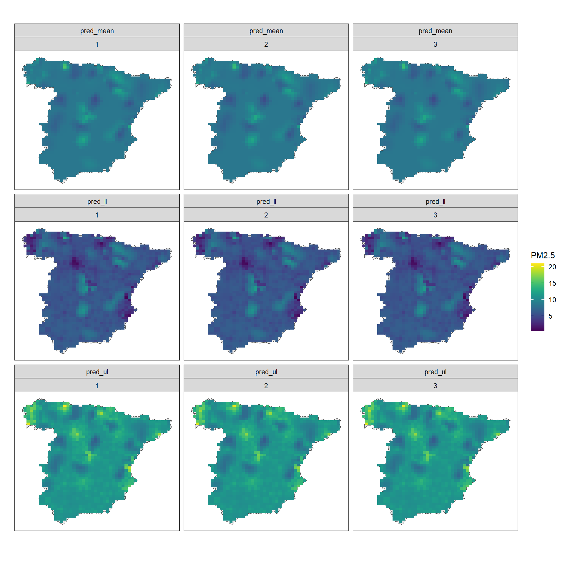
FIGURE 10.12: PM\(_{2.5}\) predictions and lower and upper limits of 95% CI in Spain in years 2015, 2016 and 2017.
Note that in addition to the air pollution mean and 95% credible intervals, we can also calculate the probabilities that air pollution exceeds a threshold value that is relevant for policymaking. Examples on how to calculate exceedance probabilities are given in Chapters 4, 6 and 9.