1 Simple linear regression
Learning objectives
- Correlation
- Simple linear regression example
1.1 Regression and correlation
A regression model describes the linear relationship between a response variable and one or more explanatory variables
In simple linear regression there is one explanatory variable
Example: How does body mass index relate to physical activity?
In multiple linear regression there is more than one explanatory variable
Example: How does systolic blood pressure relate to age and weight?
In correlation analysis we assess the linear association between two variables when there is no clear response-explanatory relationship
Example: What is the correlation between arm length and leg length?
1.2 Correlation
The Pearson correlation \(r\) gives a measure of the linear relationship between two variables \(x\) and \(y\).
Given a set of observations \((x_1, y_1), (x_2,y_2), \ldots, (x_n,y_n)\), the correlation between \(x\) and \(y\) is given by
\[r = \frac{1}{n-1} \sum_{i=1}^n \left(\frac{x_i-\bar x}{s_x}\right) \left(\frac{y_i-\bar y}{s_y}\right),\] where \(\bar x\), \(\bar y\), \(s_x\) and \(s_y\) are the sample means and standard deviations for each variable.
Sample variances: \(s^2_x = \frac{1}{n-1} \sum_{i=1}^n (x_i - \bar x)^2,\ \ s^2_y = \frac{1}{n-1} \sum_{i=1}^n (y_i - \bar y)^2\).
Sample covariance \(s_{xy} = \frac{1}{n-1} \sum_{i=1}^n (x_i - \bar x)(y_i - \bar y)\).
Sample correlation \(r_{xy} = \frac{s_{xy}}{s_x s_y}\).
\[-1\leq r \leq 1\]
- \(r=-1\) is total negative correlation (increasing values in one variable correspond to decreasing values in the other variable)
- \(r=0\) is no correlation (there is not linear correlation between the variables)
- \(r=1\) is total positive correlation (increasing values in one variable correspond to increasing values in the other variable)
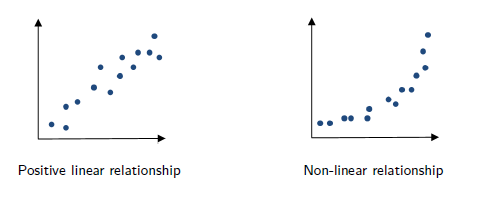
Correlation describes only the linear part of a relationship. It does not describe curved relationships.
Example
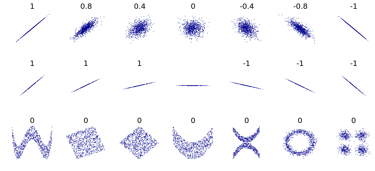
What is the correlation coefficients for these data sets?
![]()
Solution
1.3 Simple Linear Regression. BMI and physical activity
- Researchers are interested in the relationship between physical activity (PA) measured with a pedometer and body mass index (BMI)
- A sample of 100 female undergraduate students were selected. Students wore a pedometer for a week and the average steps per day (in thousands) was recorded. BMI (kg/m\(^2\)) was also recorded.
- Is there a statistically significant linear relationship between physical activity and BMI? If so, what is the nature of the relationship?
Read data
First rows of data
Summary data
##     SUBJECT             PA              BMI
##  Min.   :  1.00   Min.   : 3.186   Min.   :14.20
##  1st Qu.: 25.75   1st Qu.: 6.803   1st Qu.:21.10
##  Median : 50.50   Median : 8.409   Median :24.45
##  Mean   : 50.50   Mean   : 8.614   Mean   :23.94
##  3rd Qu.: 75.25   3rd Qu.:10.274   3rd Qu.:26.75
##  Max.   :100.00   Max.   :14.209   Max.   :35.10
Scatterplot of BMI versus PA

There is a lot of variation but does it look like there is a linear trend? Could the average BMI be a straight line in PA?
1.4 Regression line
- Simple linear regression investigates if there is a linear relationship between a response variable and an explanatory variable
- \(y\): response or dependent variable
- \(x\): explanatory or independent or predictor variable
- Simple linear regression fits a straight line in an explanatory variable \(x\) for the mean of a response variable \(y\)
- The fitted line is the line closest to the points in the vertical direction. It is “closest” in the sense that the sum of squares of vertical distances is minimised.

1.5 Residuals
- \(y\): observed value of the response variable for a value of the explanatory variable equal to \(x\)
- \(\hat y\): fitted or estimated mean of the response for a value of explanatory variable equal to \(x\)
- \(y - \hat y\): residual, difference between the observed and fitted values of the response for a value \(x\) of the explanatory variable
- Regression line is the line that minimizes the sum of squares of the residuals of all observations

1.6 Regression line
\[Y_i = \beta_0 + \beta_1 X_{i} + \epsilon_i,\] where the error \(\epsilon_i \sim^{iid} N(0, \sigma^2), \ i = 1,\ldots,n\).
The equation of the least-squares regression line of \(y\) on \(x\) is \[\hat y = \hat \beta_0 + \hat \beta_1 x\] \[\hat y = b_0 + b_1 x\]
\(\hat y\) is the estimated mean or expected response. \(\hat y\) estimates the mean response for any value of \(x\) that we substitute in the fitted regression line
\(b_0\) is the intercept of the fitted line. It is the value of \(\hat y\) when \(x=0\).
\(b_1\) is the slope of the fitted line. It tells how much increase (or decrease) there is for \(\hat y\) as \(x\) increases by one unit
If \(b_1>0\) \(\hat y\) increases as \(x\) increases
If \(b_1<0\) \(\hat y\) decreases as \(x\) increases
The slope \(b_1=r\frac{s_y}{s_x} = \frac{s_{xy}}{s_x s_y}\frac{s_y}{s_x} = \frac{s_{xy}}{s^2_x} = \frac{\sum(x_i - \bar x)(y_i-\bar y)}{\sum (x_i - \bar x)^2}\) and the intercept \(b_0 = \bar y - b_1 \bar x\)
Here \(r\) is the correlation which gives a measure of the linear relationship between \(x\) and \(y\)
\[-1\leq r \leq 1\]
- \(r=-1\) is total negative correlation
- \(r=0\) is no correlation
- \(r=1\) is total positive correlation

After fitting the model it is crucial to check whether the model assumptions are valid before performing inference. If there is any assumption violation, subsequent inferential procedures may be invalid. For example, we need to look at residuals. Are they randomly scattered so a straight line is a good model to fit?
Example
The Coast Starlight Amtrak train runs from Seattle to Los Angeles. The scatterplot below displays the distance between each stop (in miles) and the amount of time it takes to travel from one stop to another (in minutes).
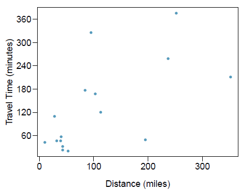
The mean travel time from one stop to the next on the Coast Starlight is 129 mins, with a standard deviation of 113 minutes. The mean distance traveled from one stop to the next is 108 miles with a standard deviation of 99 miles. The correlation between travel time and distance is 0.636.
- Write the equation of the regression line for predicting travel time.
- Interpret the slope and the intercept in this context.
- The distance between Santa Barbara and Los Angeles is 103 miles. Use the model to estimate the time it takes for the Starlight to travel between these two cities.
- It actually takes the Coast Starlight about 168 mins to travel from Santa Barbara to Los Angeles. Calculate the residual and explain the meaning of this residual value.
- Suppose Amtrak is considering adding a stop to the Coast Starlight 500 miles away from Los Angeles. Would it be appropriate to use this linear model to predict the travel time from Los Angeles to this point?
Solution
Travel time: \(\bar y= 129\)
minutes, \(s_y = 113\) minutes.
Distance: \(\bar x = 108\) miles, \(s_x= 99\) miles.
Correlation between travel time and distance \(r = 0.63\)
First calculate the slope: \(b_1 = r \times s_y/s_x = 0.636 \times 113/99 = 0.726\). Next, make use of the fact that the regression line passes through the point \((\bar x, \bar y)\): \(\bar y = b_0+b_1 \times \bar x\). Then, \(b_0 = \bar y - b_1 \bar x = 129 - 0.726 \times 108 = 51\).
\(\widehat{\mbox{travel time}} = 51 + 0.726 \times \mbox{distance}\).\(b_1\): For each additional mile in distance, the model predicts an additional 0.726 minutes in mean travel time.
\(b_0\): When the distance traveled is 0 miles, the travel time is expected to be 51 minutes. It does not make sense to have a travel distance of 0 miles in this context. Here, the y-intercept serves only to adjust the height of the line and is meaningless by itself.\(\widehat{\mbox{travel time}} = 51 + 0.726 \times \mbox{distance} = 51+0.726 \times 103 \approx 126\) minutes.
(Note: we should be cautious in our predictions with this model since we have not yet evaluated whether it is a well-fit model).\(e_i = y_i - \hat y_i = 168-126=42\) minutes. A positive residual means that the model underestimates the travel time.
I would not be appropriate since this calculation would require extrapolation.
1.7 Coefficients of the regression line
##
## Call:
## lm(formula = BMI ~ PA, data = d)
##
## Residuals:
##     Min      1Q  Median      3Q     Max
## -7.3819 -2.5636  0.2062  1.9820  8.5078
##
## Coefficients:
##             Estimate Std. Error t value Pr(>|t|)
## (Intercept)  29.5782     1.4120  20.948  < 2e-16 ***
## PA           -0.6547     0.1583  -4.135  7.5e-05 ***
## ---
## Signif. codes:  0 '***' 0.001 '**' 0.01 '*' 0.05 '.' 0.1 ' ' 1
##
## Residual standard error: 3.655 on 98 degrees of freedom
## Multiple R-squared:  0.1485, Adjusted R-squared:  0.1399
## F-statistic: 17.1 on 1 and 98 DF, p-value: 7.503e-05- \(\hat y = b_0 + b_1 x\)
- \(\widehat{BMI} = 29.58 + (- 0.65) PA\)
- \(b_0= 29.58\) is the mean value of BMI when \(PA=0\)
- \(b_1= - 0.65\) means the mean value of BMI decreases by 0.65 for every unit increase in PA
1.8 Tests for coefficients. t test
The most important test is whether the slope is 0 or not. If the slope is 0, then there is no linear relationship. Test null hypothesis ‘response variable \(y\) is not linearly related to variable \(x\)’ versus alternative hypothesis ‘\(y\) is linearly related to \(x\)’.
\(H_0: \beta_1 =0\)
\(H_1: \beta_1 \neq 0\)Test statistic: t-value = estimate of the coefficient / SE of coefficient
\[T = \frac{b_1 - 0}{SE_{b_1}}\]
- Distribution: t distribution with degrees of freedom = number of observations - 2 (because we are fitting an intercept and a slope)
\[T \sim t(n-2)\]
p-value: probability of obtaining a test statistic as extreme or more extreme than the observed, assuming the null is true.
\(H_1: \beta_1 \neq 0\). p-value is \(P(T\geq |t|)\)
##               Estimate Std. Error   t value     Pr(>|t|)
## (Intercept) 29.5782471  1.4119783 20.948089 5.706905e-38
## PA          -0.6546858  0.1583361 -4.134784 7.503032e-05
In the example p-value=7.503032e-05. There is strong evidence to suggest slope is not zero. There is strong evidence to suggest PA and BMI are linearly related.
Output also gives test for intercept. This tests the null hypothesis the intercept is 0 versus the alternative hypothesis the intercept is not 0. Usually we are not interested in this test.
1.9 Confidence interval for the slope \(\beta_1\)
A \((c)\times 100\)% (or \((1-\alpha)\times 100\)%) confidence interval for the slope \(\beta_1\) is \[b_1 \pm t^* \times SE_{b_1}\]
\(t^*\) is the value on the \(t(n-2)\) density curve with area \(c\) between the critical points \(-t^*\) and \(t^*\). Equivalently, \(t^*\) is the value such that \(\alpha/2\) of the probability in the \(t(n-2)\) distribution is below \(t^*\).
1.10 ANOVA. F test
##
## Call:
## lm(formula = BMI ~ PA, data = d)
##
## Residuals:
##     Min      1Q  Median      3Q     Max
## -7.3819 -2.5636  0.2062  1.9820  8.5078
##
## Coefficients:
##             Estimate Std. Error t value Pr(>|t|)
## (Intercept)  29.5782     1.4120  20.948  < 2e-16 ***
## PA           -0.6547     0.1583  -4.135  7.5e-05 ***
## ---
## Signif. codes:  0 '***' 0.001 '**' 0.01 '*' 0.05 '.' 0.1 ' ' 1
##
## Residual standard error: 3.655 on 98 degrees of freedom
## Multiple R-squared:  0.1485, Adjusted R-squared:  0.1399
## F-statistic: 17.1 on 1 and 98 DF, p-value: 7.503e-05- In simple linear regression, this is doing the same test as the t test. Test null hypothesis ‘response variable \(y\) is not linearly related to variable \(x\)’ versus alternative hypothesis ‘\(y\) is linearly related to \(x\)’.
- The p-value is the same.
- We will look at ANOVA in multiple regression.
1.11 R\(^2\) in simple linear regression
- R\(^2\) (R-squared or coefficient of determination) is the proportion of variation of the response variable \(y\) that is explained by the model.
\[R^2 = \frac{\mbox{variability explained by the model}}{\mbox{total variability}} = \frac{\sum_{i=1}^n (\hat y_i - \bar y)^2}{\sum_{i=1}^n ( y_i - \bar y)^2}\]
or equivalently
\[R^2 = 1 - \frac{\mbox{variability in residuals}}{\mbox{total variability}} = 1 - \frac{\sum_{i=1}^n ( y_i - \hat y_i)^2}{\sum_{i=1}^n ( y_i - \bar y)^2}\]
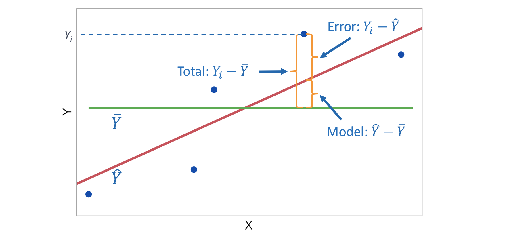
R\(^2\) measures how successfully the regression explains the response.
If the data lie exactly on the regression line then R\(^2\) = 1.
If the data are randomly scattered or in a horizontal line then R\(^2\) = 0.
For simple linear regression, R\(^2\) is equal to the square of the correlation between response variable \(y\) and explanatory variable \(x\). \[R^2 = r^2\]
Remember the correlation \(r\) gives a measure of the linear relationship between \(x\) and \(y\)
\[-1\leq r \leq 1\]
- \(r=-1\) is total negative correlation
- \(r=0\) is no correlation
- \(r=1\) is total positive correlation
\(R^2\) will increase as more explanatory variables are added to a regression model. We look at R\(^2\)(adj).
R\(^2\)(adj) or Adjusted R-squared is the proportion of variation of the response variable explained by the fitted model adjusting for the number of parameters.
- In the example R\(^2\)(adj)=13.99%. The model explains about 14% of the variation of BMI adjusting for the number of parameters.
## [1] 0.13985181.12 Estimation and prediction
1.12.1 Estimation and prediction
The regression equation can be used to estimate the mean response or to predict a new response for particular values of the explanatory variable.
When PA is 10, the estimated mean of BMI is \(\widehat{BMI} = b_0 + b_1 \times 10 = 29.5782 - 0.6547 \times 10 = 23.03\).
When PA is 10, the predicted BMI of a new individual is also \(\widehat{BMI} = b_0 + b_1 \times 10 = 29.5782 - 0.6547 \times 10 = 23.03\).
Extrapolation occurs when we estimate the mean response or predict a new response for values of the explanatory variables which are not in the range of the data used to determine the estimated regression equation. In general, this is not a good thing to do.
When PA is 50, the estimated mean of BMI is \(\widehat{BMI} = b_0 + b_1 \times 50 = 29.5782 - 0.6547 \times 50 = -3.15\).
1.12.2 Confidence and prediction intervals
A confidence interval is an interval estimate for the mean response for particular values of the explanatory variables
We can calculate the 95% CI as \(\widehat{y} \pm t^* \times SE(\widehat{y})\) where \(t^*\) is the value such that \(\alpha/2\) probability on the t(n-2) distribution is below \(t^*\).
In R, we can calculate the 95% CI with the predict()
function and the option interval = "confidence".
new <- data.frame(PA = 10)
predict(lm(BMI ~ PA, data = d), new, interval = "confidence", se.fit = TRUE)
## $fit
## fit lwr upr
## 1 23.03139 22.18533 23.87744
##
## $se.fit
## [1] 0.4263387
##
## $df
## [1] 98
##
## $residual.scale
## [1] 3.654883## [1] 22.18533 23.87745A prediction interval is an interval estimate for an individual value of the response for particular values of the explanatory variables
We can calculate the 95% PI as \(\widehat{y}_{new} \pm t^* \times \sqrt{MSE +
[SE(\widehat{y})]^2}\) where \(t^*\) is the value such that \(\alpha/2\) probability on the t(n-2)
distribution is below \(t^*\). The
Residual standard error and $residual.scale in
the R output is equal to \(\sqrt{MSE}\).
In R, we can calculate the 95% CI with the predict()
function and the option interval = "prediction".
## $fit
##        fit      lwr      upr
## 1 23.03139 15.72921 30.33357
##
## $se.fit
## [1] 0.4263387
##
## $df
## [1] 98
##
## $residual.scale
## [1] 3.654883c(23.03139 + qt(0.05/2, 98)*sqrt(3.654883^2 + 0.4263387^2),
23.03139 - qt(0.05/2, 98)*sqrt(3.654883^2 + 0.4263387^2))## [1] 15.72921 30.33357- Prediction intervals are wider than confidence intervals because there is more uncertainty in predicting an individual value of the response variable than in estimating the mean of the response variable
- The formula for the prediction interval has the extra MSE term. A confidence interval for the mean response will always be narrower than the corresponding prediction interval for a new observation.
- The width of the intervals reflects the amount of information over the range of possible \(x\) values. We are more certain of predictions at the center of the data than at the edges. Both intervals are narrowest at the mean of the explanatory variable.
