Ordinary least squares estimator is the best linear unbiased estimator (BLUE).
\[\hat \beta_{OLS} = (X'X)^{-1}X'Y\]
\[Var(\hat \beta_{OLS}) = \sigma^2 (X'X)^{-1}\]
We have assumed that errors are independent and variance of errors is constant, \(Var(\epsilon) = \sigma^2 I\). But it can happen that errors have non-constant variance or errors are correlated. We can address the problem with Generalized least squares and Weighted least squares regression.
18.2 Generalized least squares
Suppose we know the correlation and relative variance between the errors but we do not know the absolute scales.
\[Y = X\beta + \epsilon\]
\[Var(\epsilon) = \sigma^2 \Sigma,\ \sigma^2\ \mbox{ is unknown and }\ \Sigma\ \mbox{ is known}.\]
Instead of minimizing the Residual Sum of Squares, Generalized least squares minimizes
\[(Y-X\beta)' \Sigma^{-1} (Y-X\beta)\] which is solved by
\(\Sigma\) is a symmetric positive-definite matrix which can be expressed as \(\Sigma = SS'\), where \(S\) lower triangular matrix, using Cholesky decomposition.
GLS is like regressing \(X^* = S^{-1}X\) on \(Y^* = S^{-1}Y\).
Sometimes the errors are uncorrelated, but have unequal variance where the form of the inequality is known.
When \(\Sigma\) is diagonal, the errors are uncorrelated but do not necessarily have equal variance:
\[\Sigma = \mbox{diag}(1/w_1, \ldots, 1/w_n).\]
Weighted least squares (WLS) regression is a technique that fits a regression model not by minimizing \(RSS = \sum e_i^2\) as in ordinary regression, but rather by minimizing a weighted residual sum of squares \(RSS = \sum w_i e_i^2\).
The weight \(w_i\) is chosen in such a way so that it is inversely proportional to the variance of the error \(\epsilon_i\) at that point.
Small weights where the variance is large and big weights where the variance is small.
Then, \[S = \mbox{diag}\left(\sqrt{1/w_1}, \ldots, \sqrt{1/w_n}\right),\] so we can regress \(\sqrt{w_i}x_i\) on \(\sqrt{w_i}y_i\).
WLS is easily implemented in R by using the weights option in lm().
Errors proportional to a predictor: \(Var(\epsilon_i) \propto x_i\) suggests \(w_i = x_i^{-1}\)
\(Y_i\) are the averages of \(n_i\) observations then \(Var(y_i) = Var(\epsilon_i) = \sigma^2/n_i\) suggests \(w_i = n_i\)
18.4 GLS
Let \(Y_i=\beta X_i+\epsilon_i\), \(i=1,2\), where \(\epsilon_1 \sim N(0,\sigma^2)\) and \(\epsilon_2 \sim N(0,2\sigma^2)\), and \(\epsilon_1\) and \(\epsilon_2\) are statistically independent.
If \(X_1=1\) and \(X_2=-1\), obtain \(\hat \beta\) and its variance.
GLS. Solutions
\[Var(\epsilon) = \sigma^2 \Sigma,\ \sigma^2\ \mbox{ is unknown and }\ \Sigma\ \mbox{ is known}.\]
\[\hat{\beta}=\left( X^T \Sigma^{-1} X \right)^{-1} X^T \Sigma^{-1} Y\]
Examples from Faraway (2005) Linear Models with R, Chapman & Hall/CRC
18.5.1 Generalized least squares
Longley’s regression data where the response is the number of people employed, yearly from 1947 to 1962, and the predictors are GNP (Gross National Product) implicit price deflator (1954=100), and population 14 years of age and over.
Fit model.
data(longley)g <-lm(Employed ~ GNP + Population, data = longley)summary(g)
Call:
lm(formula = Employed ~ GNP + Population, data = longley)

Residuals:
     Min       1Q   Median       3Q      Max
-0.80899 -0.33282 -0.02329  0.25895  1.08800

Coefficients:
            Estimate Std. Error t value Pr(>|t|)
(Intercept) 88.93880   13.78503   6.452 2.16e-05 ***
GNP          0.06317    0.01065   5.933 4.96e-05 ***
Population  -0.40974    0.15214  -2.693   0.0184 *
---
Signif. codes:  0 '***' 0.001 '**' 0.01 '*' 0.05 '.' 0.1 ' ' 1

Residual standard error: 0.5459 on 13 degrees of freedom
Multiple R-squared:  0.9791,    Adjusted R-squared:  0.9758
F-statistic: 303.9 on 2 and 13 DF,  p-value: 1.221e-11
In data collected over time such as this, successive errors could be correlated. Assuming errors take a simple autoregressive form:
\[\epsilon_{i+1} = \rho \epsilon_i + \delta_i\]
where \(\delta_i \sim N(0, \tau^2)\). We can estimate this correlation \(\rho\) by
cor(g$residuals[-1], g$residuals[-16])
[1] 0.3104092
Under this assumption \(\Sigma_{ij}=\rho^{|i-j|}\). For simplicity, let us assume we know that \(\rho = 0.31041\). We now construct the matrix \(\Sigma\) matrix and compute the GLS estimate of \(\beta\).
The gls() function of the nlme package can also be used to fit the model using GLS.
18.5.2 Weighted least squares
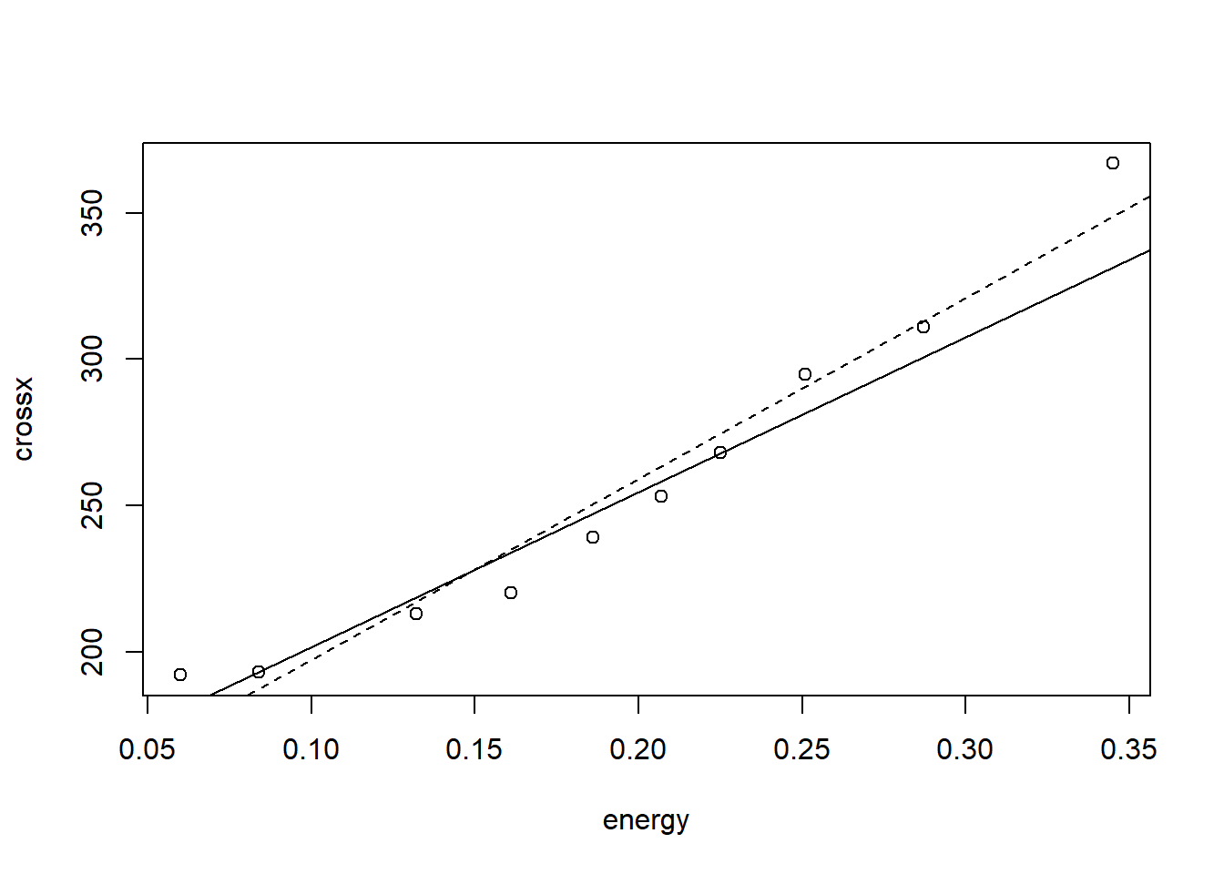
Dataset from an experiment to study the interaction of certain kinds of elementary particles on collision with proton targets. The cross-section variable is believed to be linearly related to the inverse of energy (energy has already been inverted). At each level of the momentum, a very large number of observations were taken so that is was possible to accurately estimate the standard deviation of the response (sd).
g <-lm(crossx ~ energy, data = strongx, weights = sd^{-2})
Regression without weights
gu <-lm(crossx ~ energy, data = strongx)
Comparison two fits
plot(crossx ~ energy, data = strongx)abline(g)abline(gu, lty =2)
The unweighted fit appears to fit the data better overall but remember that for lower values of energy, the variance in the response is less and so the weighted fit tries to catch these points better than the others.