Shrinkage/regularization methods(ridge and lasso regression)
19.1 Variable selection
Carefully selected variables can improve model’s fit. But adding too many can lead to overfitting:
Overfitted models describe random error or noise instead of any underlying relationship
They generally have poor predictive performance on test data
19.2 Stepwise selection
19.2.1 Backward stepwise selection
Specify \(\alpha\) to remove It does not have to necessarily be 5%.
Start with the model that contains all predictors
Remove the predictor with highest p-value greater than \(\alpha\)
Refit the model and go to 2
Stop when all p-values are less than \(\alpha\)
19.2.2 Forward stepwise selection
This just reverses the backward method.
Specify \(\alpha\) to enter It does not have to necessarily be 5%.
Start with no variables in the model.
For all predictors not in the model, check their p-value if they are added to the model. Choose the one with lowest p-value less than \(\alpha\)
Refit the model and go to 2
Continue until no new predictors can be added
19.2.3 Stepwise regression
This is a combination of backward elimination and forward selection. At each stage a variable may be added or removed and there are several variations on exactly how this is done.
This addresses the situation where variables are added or removed early in the process and we want to change our mind about them later.
Procedure
Set significance levels
Specify an \(\alpha_1\)-to-enter and \(\alpha_2\)-to-remove significance levels.
Models one predictor
Fit each of the one-predictor models. Include in the stepwise model the predictor with the smallest p-value less than \(\alpha_1\) (\(x_1\)).
Models two predictors
Fit each of the two-predictors that include \(x_1\) as predictor. Include in the stepwise model the predictor with the smallest p-value less than \(\alpha_1\) (\(x_2\)).
If no predictor has a p-value less than \(\alpha_1\), stop. The model with the one predictor obtained is the final model.
Check the p-value for testing \(\beta_1=0\). If now \(x_1\) is not significant (p-value greater \(\alpha_2\)), remove from the model.
Models three predictors
(Suppose \(x_1\) and \(x_2\) are in the model)
Fit each of the three-predictor models that include \(x_1\) and \(x_2\) as predictors. Include in the stepwise model the predictor with the smallest p-value less than \(\alpha_1\) (\(x_3\)).
If no predictor has a p-value less than \(\alpha_1\), stop. The model with the two predictors obtained is the final model.
Check the p-values for testing \(\beta_1 =0\) and \(\beta_2=0\). If now \(x_1\) or \(x_2\) are not significant (p-value greater \(\alpha_2\)), remove from the model.
Stopping the procedure
Continue the steps until adding an additional predictor does not yield a p-value less than \(\alpha_1\)
19.2.4 Example
Data on the 50 US states collected from US Bureau of the Census. Variables:
life expectancy in years (1969-71)
population estimate as of July 1, 1975
per capita income (1974)
illiteracy (1970, percent of population)
murder and non-negligent manslaughter rate per 100,000 population (1976)
percent high-school graduates (1970)
mean number of days with min temperature \(<\) 32 degrees (1931-1960) in capital or large city
land area in square miles
We take life expectancy as the response and the remaining variables as predictors.
Example backward stepwise selection. At each stage we remove the predictor with the largest p-value over 0.05.
Call:
lm(formula = Life.Exp ~ ., data = statedata)

Residuals:
     Min       1Q   Median       3Q      Max
-1.48895 -0.51232 -0.02747  0.57002  1.49447

Coefficients:
              Estimate Std. Error t value Pr(>|t|)
(Intercept)  7.094e+01  1.748e+00  40.586  < 2e-16 ***
Population   5.180e-05  2.919e-05   1.775   0.0832 .
Income      -2.180e-05  2.444e-04  -0.089   0.9293
Illiteracy   3.382e-02  3.663e-01   0.092   0.9269
Murder      -3.011e-01  4.662e-02  -6.459 8.68e-08 ***
HS.Grad      4.893e-02  2.332e-02   2.098   0.0420 *
Frost       -5.735e-03  3.143e-03  -1.825   0.0752 .
Area        -7.383e-08  1.668e-06  -0.044   0.9649
---
Signif. codes:  0 '***' 0.001 '**' 0.01 '*' 0.05 '.' 0.1 ' ' 1

Residual standard error: 0.7448 on 42 degrees of freedom
Multiple R-squared:  0.7362,    Adjusted R-squared:  0.6922
F-statistic: 16.74 on 7 and 42 DF,  p-value: 2.534e-10
g <-update(g, . ~ . - Area)summary(g)
Call:
lm(formula = Life.Exp ~ Population + Income + Illiteracy + Murder +
    HS.Grad + Frost, data = statedata)

Residuals:
     Min       1Q   Median       3Q      Max
-1.49047 -0.52533 -0.02546  0.57160  1.50374

Coefficients:
              Estimate Std. Error t value Pr(>|t|)
(Intercept)  7.099e+01  1.387e+00  51.165  < 2e-16 ***
Population   5.188e-05  2.879e-05   1.802   0.0785 .
Income      -2.444e-05  2.343e-04  -0.104   0.9174
Illiteracy   2.846e-02  3.416e-01   0.083   0.9340
Murder      -3.018e-01  4.334e-02  -6.963 1.45e-08 ***
HS.Grad      4.847e-02  2.067e-02   2.345   0.0237 *
Frost       -5.776e-03  2.970e-03  -1.945   0.0584 .
---
Signif. codes:  0 '***' 0.001 '**' 0.01 '*' 0.05 '.' 0.1 ' ' 1

Residual standard error: 0.7361 on 43 degrees of freedom
Multiple R-squared:  0.7361,    Adjusted R-squared:  0.6993
F-statistic: 19.99 on 6 and 43 DF,  p-value: 5.362e-11
g <-update(g, . ~ . - Illiteracy)summary(g)
Call:
lm(formula = Life.Exp ~ Population + Income + Murder + HS.Grad +
    Frost, data = statedata)

Residuals:
    Min      1Q  Median      3Q     Max
-1.4892 -0.5122 -0.0329  0.5645  1.5166

Coefficients:
              Estimate Std. Error t value Pr(>|t|)
(Intercept)  7.107e+01  1.029e+00  69.067  < 2e-16 ***
Population   5.115e-05  2.709e-05   1.888   0.0657 .
Income      -2.477e-05  2.316e-04  -0.107   0.9153
Murder      -3.000e-01  3.704e-02  -8.099 2.91e-10 ***
HS.Grad      4.776e-02  1.859e-02   2.569   0.0137 *
Frost       -5.910e-03  2.468e-03  -2.395   0.0210 *
---
Signif. codes:  0 '***' 0.001 '**' 0.01 '*' 0.05 '.' 0.1 ' ' 1

Residual standard error: 0.7277 on 44 degrees of freedom
Multiple R-squared:  0.7361,    Adjusted R-squared:  0.7061
F-statistic: 24.55 on 5 and 44 DF,  p-value: 1.019e-11
g <-update(g, . ~ . - Income)summary(g)
Call:
lm(formula = Life.Exp ~ Population + Murder + HS.Grad + Frost,
    data = statedata)

Residuals:
     Min       1Q   Median       3Q      Max
-1.47095 -0.53464 -0.03701  0.57621  1.50683

Coefficients:
              Estimate Std. Error t value Pr(>|t|)
(Intercept)  7.103e+01  9.529e-01  74.542  < 2e-16 ***
Population   5.014e-05  2.512e-05   1.996  0.05201 .
Murder      -3.001e-01  3.661e-02  -8.199 1.77e-10 ***
HS.Grad      4.658e-02  1.483e-02   3.142  0.00297 **
Frost       -5.943e-03  2.421e-03  -2.455  0.01802 *
---
Signif. codes:  0 '***' 0.001 '**' 0.01 '*' 0.05 '.' 0.1 ' ' 1

Residual standard error: 0.7197 on 45 degrees of freedom
Multiple R-squared:  0.736, Adjusted R-squared:  0.7126
F-statistic: 31.37 on 4 and 45 DF,  p-value: 1.696e-12
g <-update(g, . ~ . - Population)summary(g)
Call:
lm(formula = Life.Exp ~ Murder + HS.Grad + Frost, data = statedata)

Residuals:
    Min      1Q  Median      3Q     Max
-1.5015 -0.5391  0.1014  0.5921  1.2268

Coefficients:
             Estimate Std. Error t value Pr(>|t|)
(Intercept) 71.036379   0.983262  72.246  < 2e-16 ***
Murder      -0.283065   0.036731  -7.706 8.04e-10 ***
HS.Grad      0.049949   0.015201   3.286  0.00195 **
Frost       -0.006912   0.002447  -2.824  0.00699 **
---
Signif. codes:  0 '***' 0.001 '**' 0.01 '*' 0.05 '.' 0.1 ' ' 1

Residual standard error: 0.7427 on 46 degrees of freedom
Multiple R-squared:  0.7127,    Adjusted R-squared:  0.6939
F-statistic: 38.03 on 3 and 46 DF,  p-value: 1.634e-12
Exercise
Choose the best model by using forward stepwise selection.
19.3 Best subset selection
Select the subset of predictors that do the best at meeting some objective criterion such as having the largest \(R^2\) value or the smallest MSE.
Procedure:
Identify all possible regression models derived from all possible combinations of the candidate predictors. If there are \(p\) possible predictors, then there are \(2^p\) possible regression models containing the predictors.
From the possible models identified, determine the model that do the “best” at meeting some well-defined criteria.
Consider what “best” is model with:
largest \(R^2\)
largest adjusted \(R^2\)
smallest MSE
smallest AIC
smallest BIC
smallest PRESS statistic
19.3.1\(R^2\)
\[R^2 = \frac{SSM}{SST} = 1-\left(\frac{SSE}{SST}\right) = 1-\frac{\sum(Y_i-\hat Y_i)^2}{\sum(Y_i-\bar Y)^2} \]\(R^2\) can only increase as more variables are added. The model with the largest number of predictors would always win.
We can instead use the \(R^2\)-adjusted values to find the point where adding more predictors is not worthwhile, because it yields a very small increase in the \(R^2\)-value.
19.3.2 The adjusted \(R^2\), \(R^2_a\) and MSE
\(R^2_a\) is the proportion of variation of the response variable explained by the fitted model adjusting for the number of parameters.
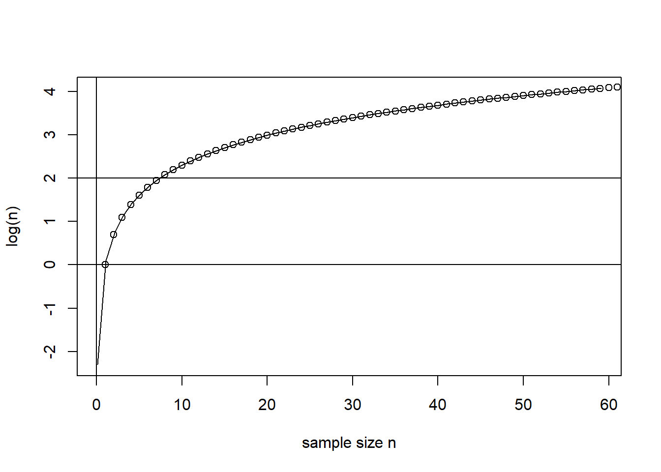
Information criterion statistics combine information about the log-likelihood, number of parameters in the model (\(p+1\), \(p\) number of predictors terms, \(p+1\) number of parameters including the intercept), and the sample size (\(n\)).
In comparing two models, the model with the lower value is preferred.
The BIC places a higher penalty on the number of parameters in the model. BIC penalizes larger models more heavily and so will tend to prefer smaller models in comparison to AIC.
19.3.4 Predicted Residual Sum of Squares PRESS
The prediction sum of squares (or PRESS) is a model validation method used to assess a model’s predictive ability that can also be used to compare regression models.
For a data set of size \(n\), PRESS is calculated by omitting each observation individually and then the remaining \(n – 1\) observations are used to calculate a regression equation which is used to predict the value of the omitted response value (which we denote by \(\hat Y_{i(-i)}\)). We then calculate the \(i\)th PRESS residual as the difference \(Y_i− \hat Y_{i(-i)}\). Then, the formula for PRESS is given by
\[PRESS = \sum_{i=1}^n (Y_i - \hat Y_{i(-i)})^2\] The smaller the PRESS, the better the model’s predictive ability.
19.3.5 Cross-validation
Holdout cross-validation:
Split the sample data into a training (or model-building) set, which we can use to develop the model, and a validation (or prediction or test) set, which is used to evaluate the predictive ability of the model. We can calculate the prediction mean squared error (pMSE) for the validation set to assess the predictive ability of the model.
where \(n_{test}\) is the size of the testing or validation data.
K-fold cross-validation:
This splits the sample dataset into \(K\) parts which are (roughly) equal in size. For each part, we use the remaining \(K–1\) parts to estimate the model of interest (i.e., the training sample) and test the predictability of the model with the remaining part (i.e., the validation sample). We then calculate the prediction mean squared errors for each part, and sum the \(K\) estimates of prediction mean squared error (pMSE) to produce a \(K\)-fold cross-validation estimate.
If \(K = n\), this is called leave-one-out cross-validation (LOOCV). That means that \(n\) separate data sets are trained on all of the data (except one point) and then prediction is made for that one point. The evaluation of this method is very good, but often computationally expensive. Note that the \(K\)-fold (\(K=n\)) cross-validation estimate of prediction mean squared error is identical to the PRESS statistic.
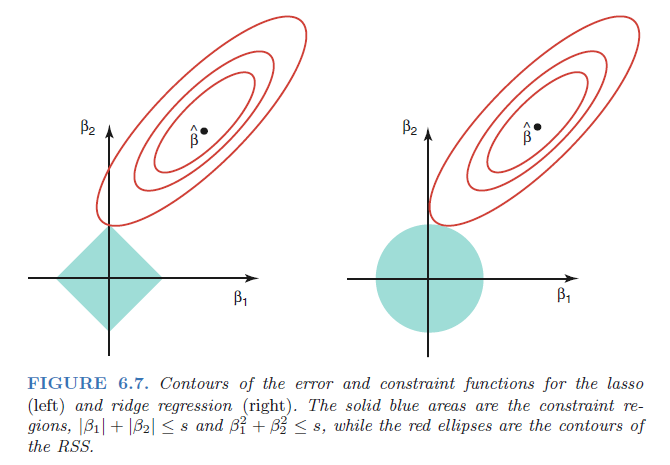
The subset selection methods described previously involve using least squares to fit a linear model that contains a subset of the predictors. As an alternative, we can fit a model containing all \(p\) predictors using a technique that constrains or regularizes the coefficient estimates, or equivalently, that shrinks the coefficient estimates towards zero.
The two best-known techniques for shrinking the regression coefficients towards zero are ridge regression and the lasso.
# Hence we see that Salary is missing for 59 players. The `na.omit()` function# removes all of the rows that have missing values in any variable.sum(is.na(Hitters$Salary))