1 Probability distributions
Learning objectives
- Random variables
- Probability distributions (Bernoulli, Binomial, normal, t, F, chi-squared, multivariate normal)
- Percentiles and quantiles
1.1 Random variables
A random process is a random phenomenon or experiment that can have a range of outcomes. For example, tossing a coin, rolling a dice, or measuring the height of a randomly selected individual.
A random variable is a variable whose possible values are numbers associated to the outcomes of a random process. Random variables are usually denoted with capital letters such as \(X\) or \(Y\). There are two types of random variables: discrete and continuous.
A discrete random variable is one which may take only a finite or countable infinite set of values. For example:
\(X =\) outcome obtained when tossing a coin (e.g., \(X=1\) if heads and \(X = 0\) if tails)
\(X =\) number of members in a family randomly selected in USA (e.g., 1, 2, 3)
\(X =\) number of patients admitted in a hospital in a given day
\(X =\) number of defective light bulbs in a box of 20
\(X =\) year that a student randomly selected in the University was born (e.g., 1998, 2000)
A continuous random variable is one which takes an infinite non-countable number of possible values. For example:
\(X\) = height of a student randomly selected in the department (e.g., 1.65 m, 1.789 m)
\(X\) = time required to run 1 Km (e.g., 4.56 min, 5.123 min)
\(X\) = amount of sugar in an orange (e.g., 9.21 g, 12.2 g)
1.2 Probability distribution
A probability distribution of a random variable \(X\) is the specification of all the possible values of \(X\) and the probability associated with those values.
1.2.1 Probability mass function
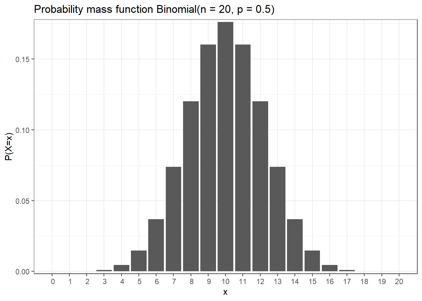
If \(X\) is discrete, the probability distribution is called probability mass function. We can describe the probability mass function of \(X\) by making a table with all the possible values of \(X\) and their associated probabilities. We can also represent graphically the probability mass function using a barplot.
Let \(X\) be a discrete random variable that may take \(n\) different values \(X = x_i\) with probability \(P(X = x_i) = p_i\), \(i =1,\ldots,n\). The probability mass function of \(X\) can be represented as follows:
| Value of \(X\) | \(P(X = x_i)\) |
|---|---|
| \(x_1\) | \(p_1\) |
| \(x_2\) | \(p_2\) |
| … | |
| \(x_n\) | \(p_n\) |
The probability mass function must satisfy the following:
- \(0 < p_i < 1\) for all \(i\)
- \(\sum_{i=1}^n p_i = p_1 + p_2 + \ldots + p_n = 1\)
Example
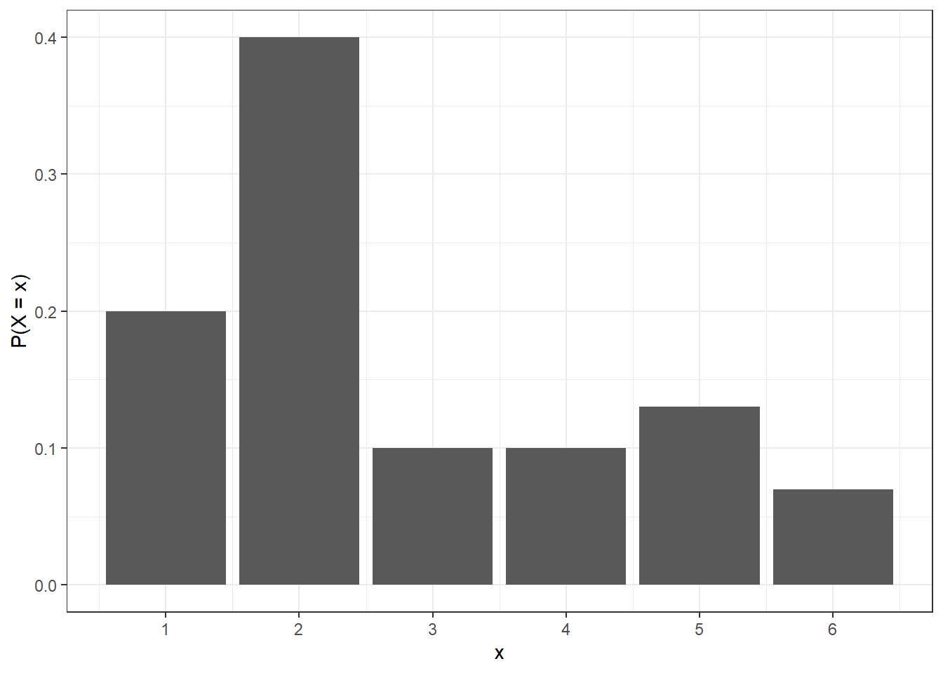
Let \(X\) be a discrete random variable with the following probability mass function.
| - | ||||||
|---|---|---|---|---|---|---|
| Outcome | 1 | 2 | 3 | 4 | 5 | 6 |
| Probability | 0.20 | 0.40 | 0.10 | 0.10 | 0.13 | 0.07 |
- Check the validity of the probability mass function.
Probabilities between 0 and 1 and sum to 1.
- Calculate the probability that \(X\) is equal to 2 or 3.
P(X = 2 or X = 3) = P(X = 2) + P(X = 3) = 0.4 + 0.1 = 0.5.
- Calculate the probability that \(X\) is greater than 1
P(X > 1) = 1 - P(X = 1) = 1 - 0.2 = 0.8
1.2.2 Probability density function
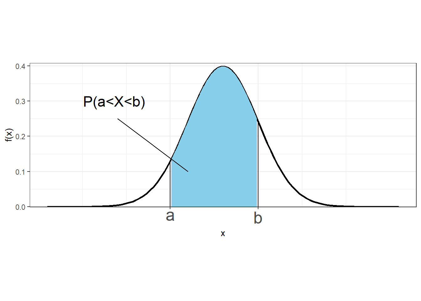
If \(X\) is continuous, the probability distribution is called probability density function. A continuous variable \(X\) takes an infinite number of possible values, and the probability of observing any single value is equal to 0 (\(P(X = x) = 0\)).
Therefore, instead of discussing the probability of \(X\) at a specific value \(x\), we deal with \(f(x)\), the probability density function of \(X\) at \(x\).
We cannot work with probabilities of \(X\) at specific values, but we can assign probabilities to intervals of values. The probability of \(X\) being between \(a\) and \(b\) is given by the area under the probability density curve from \(a\) to \(b\).
\[P(a \leq X\leq b) = \int_a^b f(x)dx\]
The probability density function \(f(x)\) must satisfy the following:
- The probability density function has no negative values (\(f(x) \geq 0\) for all \(x\))
- Total area under the curve is equal to 1 (\(\int_{-\infty}^{-\infty} f(x)dx = 1\))
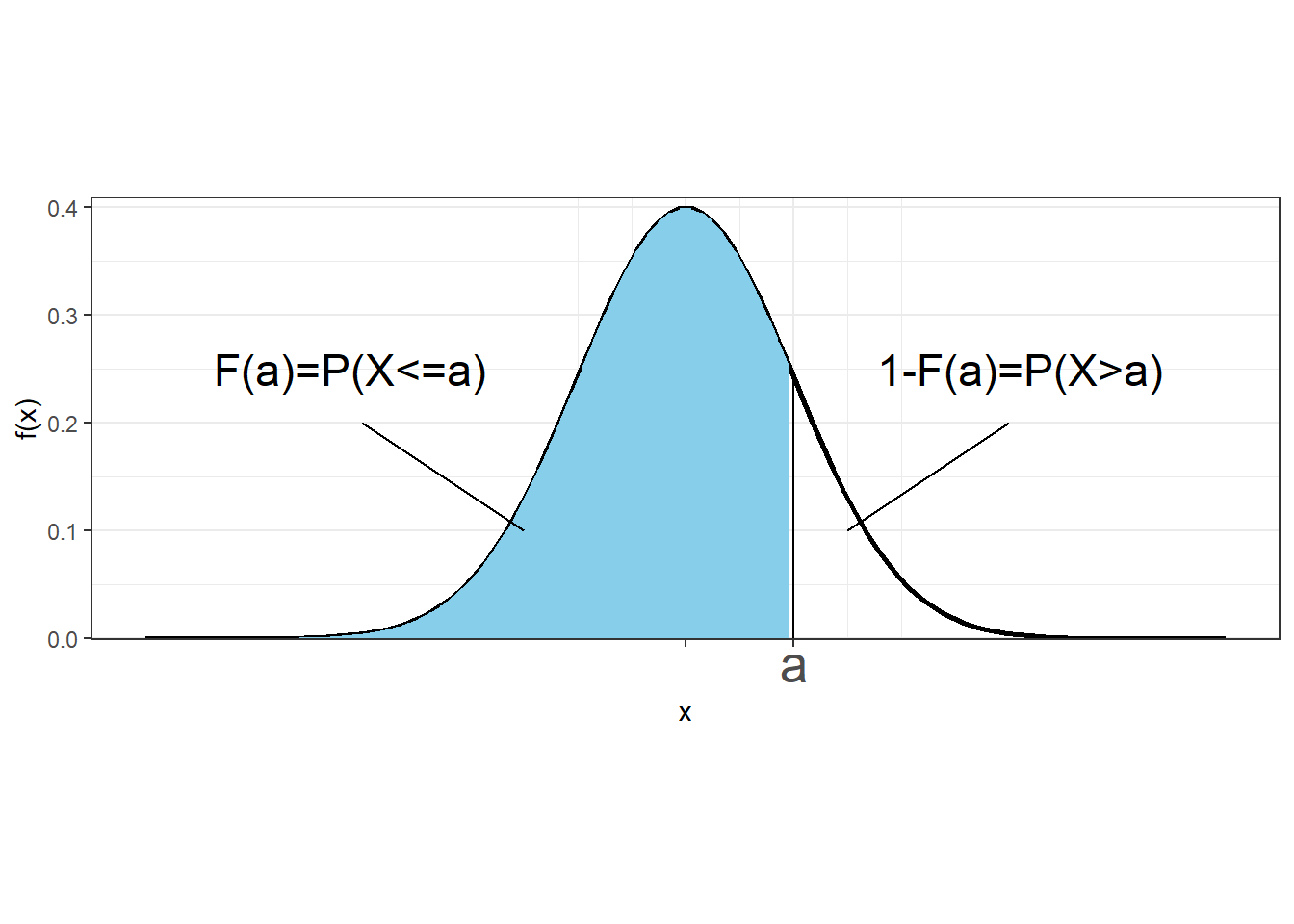
1.3 Cumulative distribution function
The cumulative distribution function (CDF) of a random variable \(X\) denotes the probability that \(X\) takes a value less than or equal to \(x\), for every value of \(x\).
If \(X\) is discrete, the cumulative distribution function at a value \(x\) is calculated as the sum of the probabilities of the values that are less than or equal to \(x\):
\[F(x)=P(X\leq x) = \sum_{a\leq x}P(X=a)\]
If \(X\) is continuous, the cumulative distribution function at value \(x\) is calculated as the area under the probability density function to the left of \(x\).
\[F(x)=P(X\leq x) = \int_{-\infty}^x f(a)da\]
The probability that a continuous variable takes values between \(a\) and \(b\) can be expressed as \(P(a \leq X \leq b) = F(b) - F(a)\)

Example
Calculate and represent graphically the cumulative distribution function for the discrete random variable given by the following probability mass function:
| - | ||||||
|---|---|---|---|---|---|---|
| Outcome | 1 | 2 | 3 | 4 | 5 | 6 |
| Probability | 0.20 | 0.40 | 0.10 | 0.10 | 0.13 | 0.07 |
\(F(1) = P(X \leq 1) = 0.20\)
\(F(2) = P(X \leq 2) = 0.20+0.40 = 0.60\)
\(F(3) = P(X \leq 3) = 0.20+0.40+0.10 = 0.70\)
\(F(4) = P(X \leq 4) = 0.20+0.40+0.10+0.10=0.80\)
\(F(5) = P(X \leq 5) = 0.20+0.40+0.10+0.10+0.13=0.93\)
\(F(6) = P(X \leq 6) = 0.20+0.40+0.10+0.10+0.13+0.07=1\)
1.4 Bernoulli distribution
The Bernoulli distribution is used to describe experiments having exactly two outcomes (e.g., the toss of a coin will be head or tail, a person will test positive for a disease or not, or a political party will win an election or not).
If \(X\) is a random variable that has a Bernoulli distribution with probability of success \(p\), we write \[X \sim Ber(p)\]
Trial can result in two possible outcomes, namely, success (\(X=1\)) and failure (\(X=0\))
Probability of success \(p\) is the same for each trial (\(0 < p < 1\))
The outcome of one trial has no influence on later outcomes (trials are independent)
Probability mass function: \[P(X = x) = p^x (1-p)^{1-x},\ x \in \{0, 1\}\]
We can check this: if \(x=0\), \(P(X=0) = p^0 (1-p)^{1-0}=1-p\), and if \(x=1\), \(P(X=1) = p^1 (1-p)^{0}=p\)Mean is \(E[X]= \sum_{i} x_i P(X=x_i) = 0 (1-p)+ 1 p=p\)
Variance is \(Var[X] = E[(X-E[X])^2] = E[X^2]-E[X]^2 = 0^2 (1-p)+ 1^2 p - p^2 = p(1-p)\)
Example
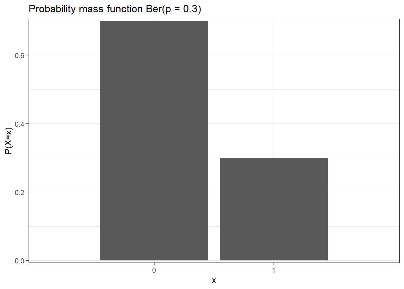
  x   y
1 0 0.7
2 1 0.3
1.5 Binomial distribution
The binomial distribution is used to describe the number of successes in a fixed number of independent Bernoulli trials (e.g., number of heads when tossing a coin 20 times, number of people that test positive for a disease out of 100 people tested (assuming trials are independent. For example, non-infectious disease))
If \(X\) is a random variable that has a Binomial distribution with number of trials \(n\) and probability of success on a single trial \(p\), we write
\[X \sim Binomial(n,p)\]
\(x=0,1,2,\ldots,n\) number of successes
The number of trials is \(n\) fixed
The probability of success \(p\) is the same from one trial to another
Each trial is independent (none of the trials have an effect on the probability of the next trial)
Probability mass function. Probability of having \(x\) successful outcomes in an experiment of \(n\) independent trials and probability of success \(p\): \[P(X=x) = \binom{n}{x} p^x (1-p)^{n-x}\]
\(x\) successes occur with probability \(p^x\) and \(n -x\) failures occur with probability \((1 - p)^{n - x}\). The \(x\) successes can occur anywhere among the \(n\) trials. There are \(\binom{n}{x}\) (\(n\) choose \(x\)) number of ways to get \(x\) successes in a sequence of \(n\) trials. \(\displaystyle{\binom{n}{x} = \frac{n!}{x!(n-x)!}}\) where \(n\) factorial = \(n! = n \times (n-1) \times \ldots \times 1\).Mean is \(n p\). Variance is \(n p (1-p)\)
Example
    x            y
1   0 9.536743e-07
2   1 1.907349e-05
3   2 1.811981e-04
4   3 1.087189e-03
5   4 4.620552e-03
6   5 1.478577e-02
7   6 3.696442e-02
8   7 7.392883e-02
9   8 1.201344e-01
10  9 1.601791e-01
11 10 1.761971e-01
12 11 1.601791e-01
13 12 1.201344e-01
14 13 7.392883e-02
15 14 3.696442e-02
16 15 1.478577e-02
17 16 4.620552e-03
18 17 1.087189e-03
19 18 1.811981e-04
20 19 1.907349e-05
21 20 9.536743e-07
1.5.1 Binomial variable is the sum of iid Bernoulli variables
A Binomial random variable is the sum of independent, identically distributed Bernoulli random variables.
Let \(X_1, X_2, \ldots, X_n\) be independent Bernoulli random variables, each with the same parameter \(p\). Then the sum \(X = X_1 + \ldots + X_n\) is a Binomial random variable with parameters \(n\) and \(p\).
Example
Suppose that a fair coin is tossed 3 times and the probability of head is \(p\). The probability of obtaining 2 heads in the first two tosses and 1 tail in the third toss is \[P(X_1 = 1, X_2 =1, X_3 = 0) = p \times p \times (1-p) = p^2 (1-p)\] (tosses are independent and probabilities are multiplied)
There are 3 possible ways we obtain 2 heads and 1 tail in three tosses:
\(P\left(\sum_{i=1}^3 X_i = 2\right) =\)
\(P(X_1 = 1, X_2 =1, X_3 = 0) + P(X_1 = 1, X_2 =0, X_3 = 1) + P(X_1 = 0, X_2 =1, X_3 = 1) =\)
\(3 p^2 (1-p)\)In general, the probability of obtaining \(x\) heads in \(n\) tosses is \[P\left(\sum_{i=1}^n X_i = x\right) = \binom{n}{x} p^x (1-p)^{n-x}\]
1.5.2 R syntax
| Purpose | Function | Example |
|---|---|---|
Generate n random values from a Binomial distribution |
rbinom(n, size, prob) |
rbinom(1000, 12, 0.25) generates 1000 values from a Binomial distribution with number of trials 12 and probability of success 0.25 |
| Probability Mass Function | dbinom(x, size, prob) |
dbinom(2, 12, 0.25) probability of obtaining 2 successes when the number of trials is 12 and the probability of success is 0.25 |
| Cumulative Distribution Function (CDF) | pbinom(q, size, prob) |
pbinom(2, 12, 0.25) probability of observing 2 or fewer successes when the number of trials is 12 and the probability of success is 0.25 |
Quantile Function (inverse of pbinom()) |
qbinom(p, size, prob) |
qbinom(0.98, 12, 0.25) value at which the CDF of the Binomial distribution with 12 trials and probability of success 0.25 is equal to 0.98 |
Example
Let us consider a biased coin that comes up heads with probability 0.7 when tossed. Let \(X\) be the random variable denoting the number of heads obtained when the coin is tossed \(X \sim Bin(n = 10, p = 0.7)\).
- What is the probability of obtaining 4 heads in 10 tosses?
\(P(X = 4)\)
dbinom(4, size = 10, prob = 0.7)[1] 0.03675691- Calculate \(P(X \leq 4)\)
\(P(X \leq 4) = P(X = 0)+P(X = 1)+P(X = 2)+P(X = 3)+P(X = 4)\)
dbinom(0, size = 10, prob = 0.7) +
dbinom(1, size = 10, prob = 0.7) +
dbinom(2, size = 10, prob = 0.7) +
dbinom(3, size = 10, prob = 0.7) +
dbinom(4, size = 10, prob = 0.7)
[1] 0.04734899Alternatively, using the cumulative distribution function
pbinom(4, size = 10, prob = 0.7)[1] 0.04734899- Generate 3 random values from \(X \sim Bin(n = 10, p = 0.7)\)
rbinom(3, size = 10, prob = 0.7)[1] 5 6 81.6 Normal distribution
The Normal distribution is used to model many procesess in nature and industry (e.g., heights, blood pressure, IQ scores, package delivery time, stock volatility)
If \(X\) is a random variable that has a normal distribution with mean \(\mu\) and variance \(\sigma^2\), we write \[X \sim N(\mu, \sigma^2)\]
\(x \in \mathbb{R}\)
Probability density function: \(\displaystyle{f(x)=\frac{1}{\sigma \sqrt{2\pi}} exp^{-(x-\mu)^2/2 \sigma^2}}\)
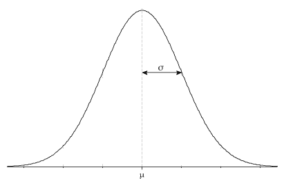
Bell-shaped density function
Single peak at the mean (most data values occur around the mean)
Symmetrical, centered at the mean
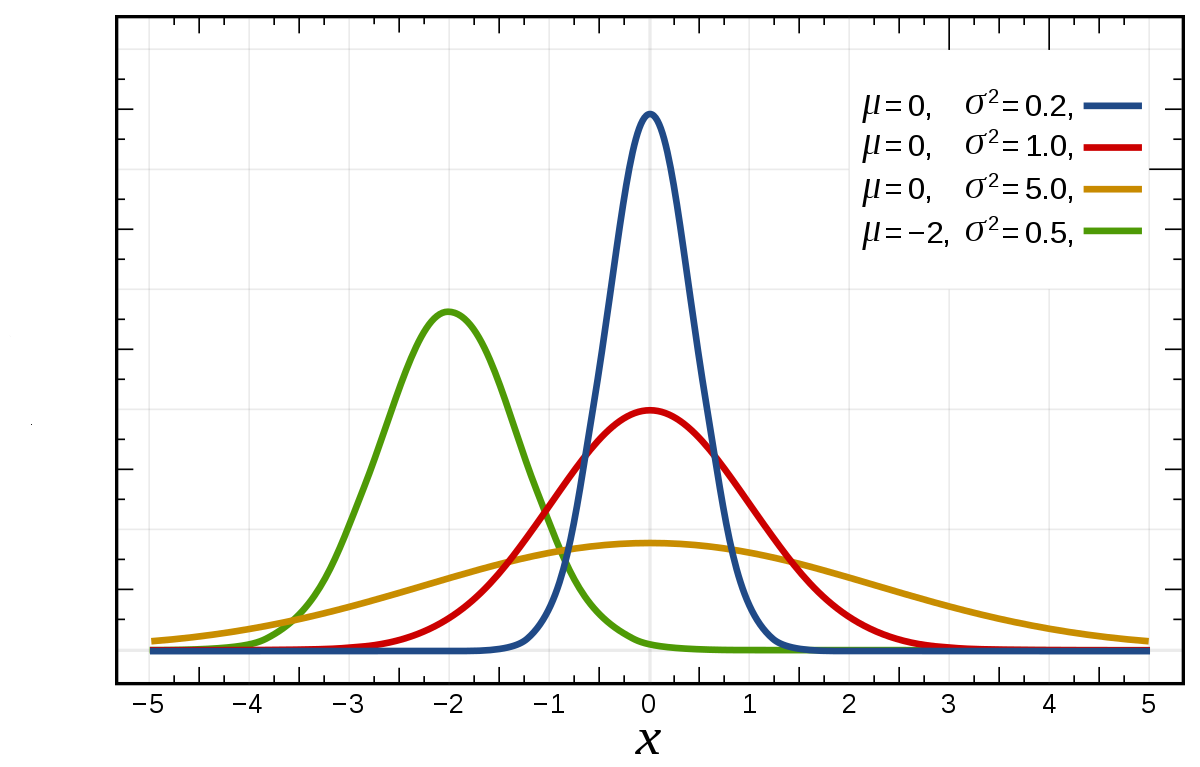
\(\mu \in \mathbb{R}\) represents the mean and the median of the normal distribution. The normal distribution is symmetric about the mean. Most values are around the mean, and half of the values are above the mean and half of the values below the mean. Changing the mean shifts the bell curve to the left or right.
\(\sigma>0\) is the standard deviation (\(\sigma^2>0\) variance). The standard deviation denotes how spread out the data are. Changing the standard deviation stretches or constricts the curve.
1.6.1 Standard Normal distribution
The standard normal distribution is a normal distribution with mean 0 and variance 1.
The standard normal distribution is represented with the letter \(Z\). \[Z \sim N(\mu=0, \sigma^2=1)\]
If \(X \sim N(\mu, \sigma^2)\), then \(\displaystyle{Z = \frac{X-\mu}{\sigma} \sim N(0, 1)}\)
1.6.2 68-95-99.7 rule
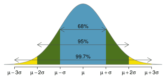
The normal distribution is symmetric about the mean \(\mu\). The total area under the probability density curve is 1. The probability below the mean is 0.5 and the probability above the mean is 0.5.
The 68-95-99.7 rule is used to remember the percentage of values that lie within a band around the mean in a normal distribution with a width of two, four and six standard deviations, respectively.
Approximately 68% of the area lies between one standard deviation below the mean (\(\mu-\sigma\)) and one standard deviation above the mean (\(\mu+\sigma\)). That is, approximately 68% of the data lies within 1 standard deviation from the mean.
Approximately 95% of the data lies within 2 standard deviations from the mean.
Approximately 99.7% of the data lies within 3 standard deviations from the mean.
1.6.3 R syntax
| Purpose | Function | Example |
|---|---|---|
Generate n random values from a Normal distribution |
rnorm(n, mean, sd) |
rnorm(1000, 2, .25) generates 1000 values from a Normal distribution with mean 2 and standard deviation 0.25 |
| Probability Density Function | dnorm(x, mean, sd) |
dnorm(0, 0, 0.5) density at value 0 (height of the probability density function at value 0) of the Normal distribution with mean 0 and standard deviation 0.5. |
| Cumulative Distribution Function (CDF) | pnorm(q, mean, sd) |
pnorm(1.96, 0, 1) area under the density function of the standard normal to the left of 1.96 (= 0.975) |
Quantile Function (inverse of pnorm()) |
qnorm(p, mean, sd) |
qnorm(0.975, 0, 1) value at which the CDF of the standard normal distribution is equal to 0.975 ( = 1.96) |
Example
Consider a random variable \(X \sim N(\mu=100, \sigma=15)\). Calculate the following:
- \(P(X < 125)\)
pnorm(125, mean = 100, sd = 15)[1] 0.9522096- \(P(X \geq 110) = 1 - P(X < 110)\)
1 - pnorm(110, mean = 100, sd = 15)[1] 0.2524925- \(P(110 < X < 125) = P(X < 125) - P(X < 110)\)
pnorm(125, mean = 100, sd = 15) -
pnorm(110, mean = 100, sd = 15)
[1] 0.20470221.7 Percentiles and quantiles
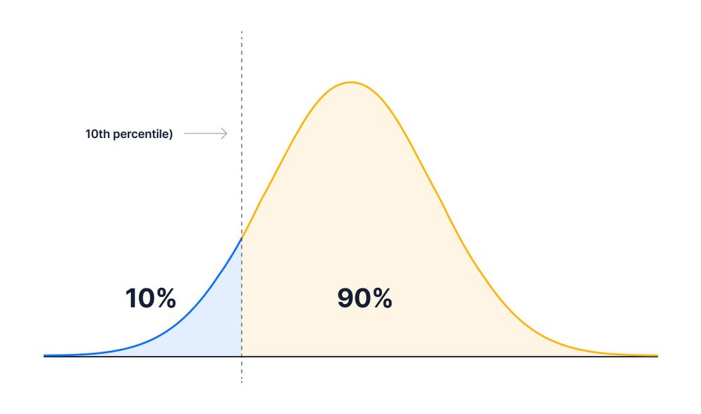
The \(k\)th percentile is the value \(x\) such that \(P(X < x) = k/100\).
The \(k\)th percentile of a set of values divides them so that \(k\)% of the values lie below and (100-\(k\))% of the values lie above.
Quantiles are the same as percentiles, but are indexed by sample fractions rather than by sample percentages (e.g., 10th percentile or 0.10 quantile).
Example
The mean Body mass index (BMI) for men aged 60 is 29 with a standard deviation of 6. Remember BMI is a value derived from the weight and height of a person to work out if weight is healthy, and it is expressed as kg/m^2.
- What is the 90th percentile (or quantile 0.90)?
\(X \sim N(\mu=29, \sigma = 6)\). The 90th percentile is the value \(x\) such that \(P(X < x) = 0.90\). The 90th percentile is 36.69. This means 90% of the BMIs in men aged 60 are below 36.69. 10% of the BMIs in men aged 60 are above 36.69.
qnorm(0.90, mean = 29, sd = 6)[1] 36.68931- Find percentile 25th (or quantile 0.25).
Value \(x\) such that \(P(X < x) = 0.25\).
qnorm(0.25, mean = 29, sd = 6)[1] 24.95306- For infant girls, the mean body length at 10 months is 72 centimeters with a standard deviation of 3 centimeters. Suppose a girl of 10 months has a measured length of 67 centimeters. How does her length compare to other girls of 10 months?
\(X \sim N(\mu=72, \sigma = 3)\). We can compute her percentile by determining the proportion of girls with lengths below 67. Specifically, \(P(X < 67) = 0.047\). This girl is in the 4.7th percentile among her peers, her height is very small.
pnorm(67, mean = 72, sd = 3)[1] 0.047790351.8 t distribution
Characteristics:
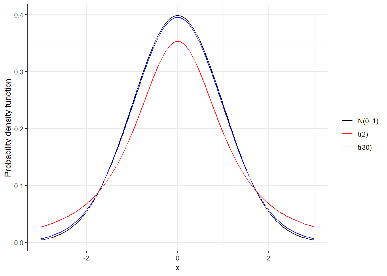
- Symmetric and bell-shaped like the normal distribution.
- Mean 0
- Heavier tails than the normal distributions, meaning observations are more likely to fall beyond two standard deviations from the mean than under the normal distribution.
The t distribution has a parameter called degrees of freedom (df). The df describes the form of the t-distribution. When the number of degrees of freedom increases, the t-distribution approaches the standard normal, N(0, 1)
R syntax
| Purpose | Function | Example |
|---|---|---|
Generate n random values from a t distribution |
rt(n, df) |
rt(1000, 2) generates 1000 values from a t distribution with 2 degrees of freedom |
| Probability Density Function (PDF) | dt(x, df) |
dt(1, 2) density at value 1 (height of the PDF at value 1) of the t distribution with 2 degrees of freedom |
| Cumulative Distribution Function (CDF) | pt(q, df) |
pt(5, 2) area under the density function of the t(2) to the left of 5 |
Quantile Function (inverse of pt()) |
qt(p, df) |
qt(0.97, 2) value at which the CDF of the t(2) distribution is equal to 0.97 |
1.9 F distribution
The F distribution is usually defined as the ratio of variances of two populations normally distributed. The F distribution depends on two parameters: the degrees of freedom of the numerator and the degrees of freedom of the denominator.
Characteristics of the F distribution:
The F-distribution is always \(\geq 0\) since it is the ratio of variances and variances are squares of deviations and hence are non-negative numbers.
Density is skewed to the right
Shape changes depending on the numerator and denominator degrees of freedom
As the degrees of freedom for the numerator and denominator get larger, the density approximates the normal
In ANOVA we always use the right-tailed area to calculate p-values
Density curves of four different F-distributions:
par(mfrow = c(2, 2)) # to draw figures in a 2 by 2 array on the device
x <- seq(0, 6, length.out = 100)
plot(x, df(x, 2, 11), main = "F(2, 11)", type = "l")
plot(x, df(x, 2, 10), main = "F(2, 10)", type = "l")
plot(x, df(x, 6, 10), main = "F(6, 10)", type = "l")
plot(x, df(x, 6, 111), main = "F(6, 111)", type = "l")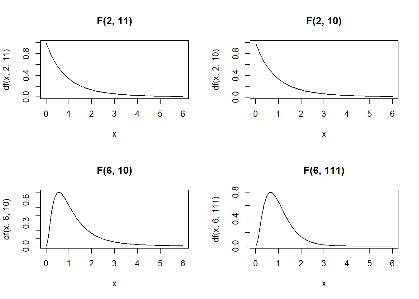
R syntax
| Purpose | Function | Example |
|---|---|---|
Generate n random values from a F distribution |
rf(n, df1, df2) |
rf(1000, 2, 11) generates 1000 values from a F distribution with degrees of freedom 2 and 11 |
| Probability Density Function (PDF) | df(x, df1, df2) |
df(1, 2, 11) density at value 1 (height of the PDF at value 1) of the F distribution with degrees of freedom 2 and 11 |
| Cumulative Distribution Function (CDF) | pf(q, df1, df2) |
pf(5, 2, 11) area under the density function of the F(2,11) to the left of 5 |
Quantile Function (inverse of pf()) |
qf(p, df1, df2) |
qf(0.97, 2, 11) value at which the CDF of the F(2,11) distribution is equal to 0.97 |
1.10 Chi-squared distribution
The chi-squared distribution with \(m \in N^*\) degrees of freedom is the distribution of a sum of squares of \(m\) independent standard normal random variables.
If \(X_1, X_2, \ldots, X_m\) are \(m\) independent random variables having the standard normal distribution, then \[V=X_1^2 + X_2^2+ \ldots + X_m^2 \sim \chi^2_{(m)}\] follows a chi-squared distribution with \(m\) degrees of freedom. Its mean is \(m\) and its variance is \(2m\).
par(mfrow = c(2, 2)) # to draw figures in a 2 by 2 array on the device
x <- seq(0, 6, length.out = 100)
plot(x, dchisq(x, 1), main = "chi2(1)", type = "l")
plot(x, dchisq(x, 2), main = "chi2(2)", type = "l")
plot(x, dchisq(x, 3), main = "chi2(3)", type = "l")
plot(x, dchisq(x, 6), main = "chi2(6)", type = "l")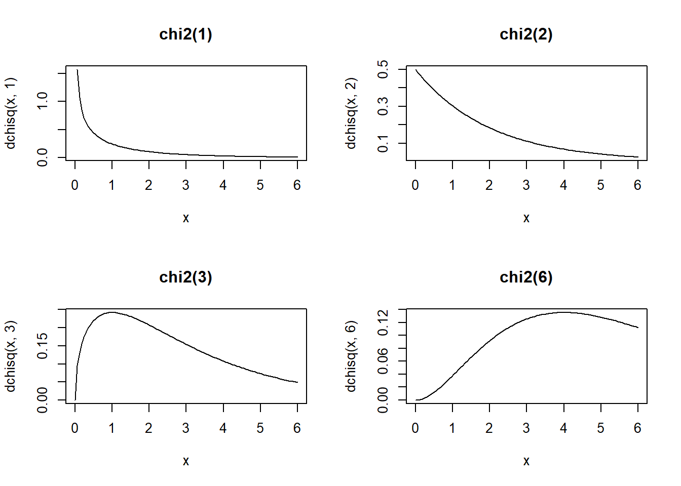
R syntax
| Purpose | Function | Example |
|---|---|---|
Generate n random values from a chi-squared distribution |
rchisq(n, df) |
rchisq(1000, 2) generates 1000 values from a chi-squared distribution with degrees of freedom 2 |
| Probability Density Function (PDF) | dchisq(x, df) |
dchisq(1, 2) density at value 1 (height of the PDF at value 1) of the chi-squared distribution with degrees of freedom 2 |
| Cumulative Distribution Function (CDF) | pchisq(q, df) |
pchisq(5, 2) area under the density function of the chi-squared(2) to the left of 5 |
Quantile Function (inverse of pchisq()) |
qchisq(p, df) |
qchisq(0.97, 2) value at which the CDF of the chi-squared(2) distribution is equal to 0.97 |
Find the 95th percentile (or quantile 0.95) of the chi-squared distribution with 6 degrees of freedom.
qchisq(0.95, df = 6)[1] 12.591591.11 Multivariate normal distribution
A vector of \(n\) random variables \(Y=(Y_1, \ldots, Y_n)'\) is said to have a multivariate normal (or Gaussian) distribution with mean \(\mu=(\mu_1, \ldots, \mu_n)'\) (\(n\times 1\)) and covariance matrix \(\Sigma\) (\(n\times n\)) (symmetric, positive definite) if its probability density function is given by
\[f(y| \mu, \Sigma) = \frac{1}{(2\pi)^{n/2}|\Sigma|^{1/2}}exp\left(-\frac{1}{2}(y-\mu)' \Sigma^{-1} (y-\mu) \right)\] We write this as \(Y \sim N(\mu, \Sigma)\)
- Shape. The contours of the joint distribution are n-dimensional ellipsoids.
- Let \(a\) be \(n\times 1\). \(Y\) is \(N(\mu, \Sigma)\) if and only if any linear combination \(a'Y\) has a (univariate) normal distribution.
- Let \(a\) be \(n\times 1\) and \(B\) be \(m \times n\). \(a' Y \sim N(a' \mu, a' \Sigma a)\), \(a+BY \sim N(a+B \mu, B \Sigma B')\)
- Let \(Z\) be \(n\) independent standard normal random variables. Then \(Y = \mu + LZ\) with \(LL'=\Sigma\) has \(N(\mu,\Sigma)\).
We can simulate multivariate normal data with the mvrnorm() function of the MASS package.
library(MASS)
library(ggplot2)

# Simulate bivariate normal data
mu <- c(0,0)                         # Mean
Sigma <- matrix(c(1, .5, .5, 1), 2)  # Covariance matrix
# > Sigma
# [,1] [,2]
# [1,]  1.0  0.5
# [2,]  0.5  1.0

# Generate sample from N(mu, Sigma)
d <- mvrnorm(5000, mu = mu, Sigma = Sigma )
head(d)
[,1] [,2]
[1,] 0.01993002 -0.6436078
[2,] 0.30715798 1.7104194
[3,] 1.46577473 -0.5476567
[4,] -0.14417368 -1.1762830
[5,] -0.32074876 -0.3702279
[6,] 0.11163699 -1.8217807ggplot(data.frame(d), aes(x = X1, y = X2)) + geom_point(alpha = .5)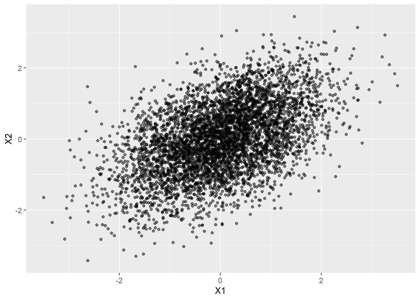
Other functions:
rmvnorm(), dmvnorm(), pmvnorm(), qmvnorm().
1.12 Distributions
Normal, chi-square, t and F distributions
Relationship between \(N\), \(\chi^2\), \(F\) and \(t\)
\(N_1, \ldots, N_s \overset{iid}{\sim} N(0,1) \rightarrow Y = N_1^2 + \ldots + N_s^2 \sim \chi_s^2\)
\(R \sim \chi^2_r\) and \(S \sim \chi^2_s\) (independent) \(\rightarrow Y=\frac{R/r}{S/s}\sim F_{r,s}\)
\(t_{df}^2 = F(1,df)\)
t distribution
A \(t_\nu\) distributed variable is a ratio of two independent random variables: a \(N(0,1)\) and the square root of a \(\chi^2_v\) divided by \(\nu\).
Let \(Z = \frac{\bar X - \mu}{\sigma/\sqrt{n}} = \sqrt{n} \frac{\bar X - \mu}{\sigma} \sim N(0,1)\)
Let \(U = \frac{(n-1)S^2}{\sigma^2} \sim \chi^2_{n-1}\)
Then,
\[T=\frac{\sqrt{n} \frac{\bar X - \mu}{\sigma}}{\sqrt{\frac{(n-1)S^2}{\sigma^2}/(n-1)}} = \frac{\sqrt{n}(\bar X - \mu)}{S} = \frac{\bar X - \mu}{S/\sqrt{n}} \sim t_{n-1}\]
F distribution
An \(F_{J,T}\) distributed variable is a ratio of two independent random variables: a \(\chi^2_J\) divided by \(J\) and a \(\chi^2_T\) divided by \(T\).
\(F = \frac{\chi^2_J/J}{\chi^2_T/T} \sim F_{J,T}\)
Let \(Z = \frac{(\bar X - \mu)}{\sigma / \sqrt{n}} = \sqrt{n}\frac{\bar X - \mu}{\sigma} \sim N(0, 1)\)
Let \(U = \frac{(n-1) S^2}{\sigma^2} \sim \chi^2_{n-1}\)
Then,
\[F = \frac{\left[\sqrt{n}\frac{(\bar{X}- \mu)}{\sigma}\right]^2/1}{\frac{(n-1)S^2}{\sigma^2}/(n-1)} = \frac{(\bar X - \mu)^2}{S^2/n} \sim F_{1, n-1}\]