(df <- 12-2-1)[1] 9qt(0.025, df)[1] -2.262157In a small study involving 12 children, the patients’ heights and weights were recorded. A catheter is passed into an artery at the femoral region and pushed up into the heart to obtain information about the heart’s physiology and functional ability. The exact catheter length required was determined. Data are reported in the table below.
| Height (in.) | Weight (lb) | Length (cm) | e^2 |
|---|---|---|---|
| 42.8 | 40.0 | 37.0 | 0.0021 |
| 63.5 | 93.5 | 49.5 | 3.3104 |
| 37.5 | 35.5 | 34.5 | 0.4175 |
| 39.5 | 30.0 | 36.0 | 2.2821 |
| 45.5 | 52.0 | 43.0 | 9.8240 |
| 38.5 | 17.0 | 28.0 | 14.5329 |
| 43.0 | 38.5 | 37.0 | 0.0406 |
| 22.5 | 8.5 | 20.0 | 49.6808 |
| 37.0 | 33.0 | 33.5 | 1.1468 |
| 23.5 | 9.5 | 30.5 | 9.3903 |
| 33.0 | 21.0 | 38.5 | 49.0623 |
| 58.0 | 79.0 | 47.0 | 0.2232 |
| \(\sum_i e_i^2 = 139.913\) |
Consider the following linear model to explain the dependence of catheter length on height and weight:
\[\mbox{length}_i = \beta_1 + \beta_2 \mbox{height}_i + \beta_3 \mbox{weight}_i + \epsilon_i\]
where the \(\epsilon_i\) are independent and Gaussian distributed as \(\epsilon_i \sim N(0, \sigma^2)\). Squared values of the residuals \(e_i\) from the model are in the table, together with their sum. For the model, \(\boldsymbol{X}\) denotes the design matrix and we have \[(\boldsymbol{X'X})^{-1} = \begin{pmatrix} 4.926 & -0.197 & 0.082\\ -0.197 & 0.008 & -0.004\\ 0.082 & -0.004 & 0.002 \end{pmatrix} \]
The least squares estimates are \(\hat \beta_1 = 21.008\), \(\hat \beta_2 = 0.196\) and \(\hat \beta_3 = 0.191\).
State the formula for computing the unbiased estimator for \(\sigma^2\). Then compute its value.
Compute the standard errors for the estimates of \(\beta_2\) and \(\beta_3\). Then construct confidence intervals for \(\beta_2\) and \(\beta_3\) using \(\alpha = 0.05\). What do you conclude?
Since \(\hat \beta = (X'X)^{-1}X' Y\) and \(Y \sim N(X\beta, \sigma^2 I)\),
\[\hat \beta \sim N(\beta, \sigma^2(X'X)^{-1})\]
\[\frac{\hat \beta_j - \beta_j}{se(\hat \beta_j)}= \frac{\hat \beta_j - \beta_j}{\sqrt{\hat \sigma^2 {{(X'X)}_{jj}^{-1}}}} \sim t_{n-p-1}\]
An unbiased estimator for \(\sigma^2\) is
\[\hat \sigma^2 = \sum_{i=1}^n \frac{(y_i-\hat y_i)^2}{n-p-1} = \sum_{i=1}^n \frac{e_i^2}{n-2-1} = \frac{139.913}{12-3}=15.547\]
Here, \(n = 12\) and the sum of residuals is given in the table \(\sum_i e_i^2 = 139.913\).
\[se(\hat \beta_j) = \hat \sigma \sqrt{{(X'X)}_{jj}^{-1}},\ \ j=1,2,3\]
\[\hat \sigma = \sqrt{\hat \sigma^2} = \sqrt{15.547} = 3.943\]
Hence by taking the square root of the second and third element on the diagonal of \({{(X'X)}_{jj}\), we have
\[se(\hat \beta_2)= 3.943 \times \sqrt{0.008} = 0.353\] \[se(\hat \beta_3) = 3.943 \times \sqrt{0.002} = 0.176\]
Confidence intervals (CI) are given by
\[\hat \beta_j \pm t_{\alpha/2, n-3}\ se(\hat \beta_j)\]
95% CI for \(\beta_2\) is \((0.196 \pm 2.262 \times 0.353) = (-0.602, 0.994)\)
95% CI for \(\beta_3\) is \((0.191 \pm 2.262 \times 0.176) = (-0.207, 0.589)\)
(df <- 12-2-1)[1] 9qt(0.025, df)[1] -2.262157Both intervals include zero. The model does not consider the effect of height and weight jointly significant in explaining the response. It might be that one or the other are separately relevant, but not when they are jointly in the model.
\[\mbox{length}_i = \beta_1 + \beta_2 \mbox{height}_i + \beta_3 \mbox{weight}_i + \epsilon_i\]
We conduct an F test to test the hypothesis
\(H_0: \beta_3 = 0\) (reduced model has intercept and height)
\(H_1: \beta_3 \neq 0\) (full model has intercept, height and also the weight covariate)
\[F=\frac{(RSS(reduced) - RSS(full))/(p_1-p_0)}{RSS(full)/(n-p_1-1)} \sim F_{p_1-p_0,\ n-p_1-1}\]
We have RSS(reduced) = 160.665 and RSS(full) = 139.913.
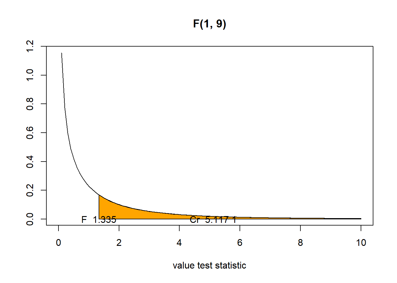
\[F_{obs} = \frac{ ( \mbox{RSS(reduced)} - \mbox{RSS(full) )}/(p_1-p_0)}{\mbox{RSS(full)}/(n-p_1-1)} = \frac{(160.665-139.913)/(2-1)}{139.913/(12-2-1)} = 1.335\]
p-value = P(F \(\geq\) F\(_{observed}\)) > \(\alpha\) = 0.05
F <- 1.335
(1 - pf(F, 1, 9))
[1] 0.27767We have \(F_{obs} = 1.335\) smaller than the critical value, quantile \(F_{0.95, 1, 9} = 5.117\).
(cr <- qf(0.95, 1, 9))[1] 5.117355Then, we fail to reject the null hypothesis \(H_0: \beta_3=0\).
We conclude there is not sufficient evidence against the null hypothesis. That is, we do not need the information carried by weight, when the height is already in the model.
Consider the regression model
\[Y_i = \beta_0 + \beta_1 X_i + \beta_2 (X_i^2-5)/4+\epsilon_i,\ i=1,\ldots,4, \] where \(\epsilon_1,\ldots,\epsilon_4\) are i.i.d. with \(E[\epsilon_i]=0\), \(Var[\epsilon_i]=\sigma^2\).
Suppose \(\boldsymbol{X}=(X_1,\ldots,X_4)' = (-3,-1,1,3)'\) and \(\boldsymbol{Y}=(Y_1,\ldots,Y_4)'=(1,2,2,4)'\).
Find the BLUE \(\boldsymbol{\hat \beta}=(\hat \beta_0, \hat \beta_1, \hat \beta_2)'\).
Based on this model, obtain a \(95\%\) CI for \(Y\) when \(X=0\). Hint: MSE = 0.45.
\[\boldsymbol{\hat{\beta}} = \boldsymbol{(X'X)^{-1} X' Y}\]
\[\boldsymbol{X}=\begin{pmatrix} 1 &-3 & 1\\ 1 &-1 & -1\\ 1 & 1 & -1\\ 1 & 3 & 1\\ \end{pmatrix}\]
\[\boldsymbol{X'X}=\begin{pmatrix} 1 &-3 & 1\\ 1 &-1 & -1\\ 1 & 1 & -1\\ 1 & 3 & 1\\ \end{pmatrix}' \begin{pmatrix} 1 &-3 & 1\\ 1 &-1 & -1\\ 1 & 1 & -1\\ 1 & 3 & 1\\ \end{pmatrix}= \begin{pmatrix} 1 & 1 & 1 & 1\\ -3 & -1 & 1 & 3\\ 1 & -1 & -1 & 1\\ \end{pmatrix} \begin{pmatrix} 1 &-3 & 1\\ 1 &-1 & -1\\ 1 & 1 & -1\\ 1 & 3 & 1\\ \end{pmatrix}= \begin{pmatrix} 4 &0 & 0\\ 0 &20 & 0\\ 0 & 0 & 4\\ \end{pmatrix} = 4 \begin{pmatrix} 1 & 0 & 0\\ 0 & 5 & 0\\ 0 & 0 & 1\\ \end{pmatrix}\\ \]
\[ \boldsymbol{(X'X)^{-1}}=\frac{1}{4} \begin{pmatrix} 1 & 0 & 0\\ 0 & 1/5 & 0\\ 0 & 0 & 1\\ \end{pmatrix}\\ \]
\[ \boldsymbol{X'Y}=\begin{pmatrix} 1 &-3 & 1\\ 1 &-1 & 1\\ 1 & 1 & -1\\ 1 & 3 & -1\\ \end{pmatrix}' \begin{pmatrix} 1 \\ 2 \\ 2 \\ 4\\ \end{pmatrix} = \begin{pmatrix} 1 & 1 & 1 & 1\\ -3 & -1 & 1 & 3\\ 1 & -1 & -1 & 1\\ \end{pmatrix} \begin{pmatrix} 1 \\ 2 \\ 2 \\ 4\\ \end{pmatrix}= \begin{pmatrix} 9 \\ 9 \\ 1 \\ \end{pmatrix}\\ \]
\[
\boldsymbol{\hat \beta}= \boldsymbol{(X'X)^{-1} X'Y} = \frac{1}{4} \begin{pmatrix}
1 & 0 & 0\\
0 & 1/5 & 0\\
0 & 0 & 1\\
\end{pmatrix} \begin{pmatrix}
9 \\
9 \\
1 \\
\end{pmatrix} =\begin{pmatrix}
9/4 \\
9/20 \\
1/4 \\
\end{pmatrix}
\]
\((1-\alpha)100\%\) confidence interval:
\[\hat Y_0 \pm t_{n-p-1, \alpha/2} \times se(\hat Y_0),\] where
\(\hat Y_0 = \boldsymbol{X_0' \hat \beta}\)
\(Var(\hat Y_0) = \boldsymbol{X'_0} Var(\boldsymbol{\hat \beta}) \boldsymbol{X_0} = \sigma^2 \boldsymbol{X_0' (X'X)^{-1} X_0}\)
\(se(\hat Y_0) = \sqrt{MSE\ \boldsymbol{X_0'(X'X)^{-1} X_0}}\)
\[\mbox{When } X = 0,\ \ \boldsymbol{X_0'}=\left(1,0,\frac{-5}{4}\right)\]
\[\hat Y_0 = \boldsymbol{X_0' \hat \beta} = 1\left(\frac{9}{4}\right)+0\left(\frac{9}{20}\right)- \frac{5}{4}\left(\frac{1}{4}\right)=\frac{31}{16} \]
\[\boldsymbol{X_0' (X'X)^{-1} X_0} = (1,0,-5/4) \left(\begin{pmatrix} 1 &-3 & 1\\ 1 &-1 & 1\\ 1 & 1 & -1\\ 1 & 3 & -1\\ \end{pmatrix}' \begin{pmatrix} 1 &-3 & 1\\ 1 &-1 & 1\\ 1 & 1 & -1\\ 1 & 3 & -1\\ \end{pmatrix}\right)^{-1} \begin{pmatrix} 1 \\ 0 \\ -5/4 \\ \end{pmatrix}= 1/4 \times 41/16\]
\[\mbox{The } 95\% \mbox{ CI is }\ \frac{31}{16} \pm \underbrace{t_{(n-p-1),1-\frac{\alpha}{2}}}_{=12.71}\sqrt{0.45\left(\frac{1}{4}\right)\left(\frac{41}{16}\right)}=\frac{31}{16} \pm 6.82 = (-4.89,8.76) \]
# n = 4, p = 2, n-p-1 = 1
qt(0.025, 1)
[1] -12.7062In 1929, Edwin Hubble investigated the relationship between the distance of a galaxy from the earth and the velocity with which it appears to be receding. Galaxies appear to be moving away from us no matter which direction we look. His paper records the distance (in megaparsecs) measured to 24 nebulae which lie outside our galaxy. For each of these nebulae Hubble also measured the velocity of the nebulae away from the earth (negative numbers mean the nebula is moving towards the earth).
distance <- c(0.032, 0.034, 0.214, 0.263, 0.275, 0.275, 0.45, 0.5,
0.5, 0.63, 0.8, 0.9, 0.9, 0.9, 0.9, 1,
1.1, 1.1, 1.4, 1.7, 2, 2, 2, 2)

velocity <- c(170, 290, -130, -70, -185, -220, 200, 290,
270, 200, 300, -30, 650, 150, 500, 920,
450, 500, 500, 960, 500, 850, 800, 1090)

d <- data.frame(velocity = velocity, distance = distance)
res <- lm(velocity ~ distance, data = d)
summary(res)
Call:
lm(formula = velocity ~ distance, data = d)

Residuals:
    Min      1Q  Median      3Q     Max
-397.96 -158.10  -13.16  148.09  506.63

Coefficients:
            Estimate Std. Error t value Pr(>|t|)
(Intercept)   -40.78      83.44  -0.489     0.63
distance      454.16      75.24   6.036 4.48e-06 ***
---
Signif. codes:  0 '***' 0.001 '**' 0.01 '*' 0.05 '.' 0.1 ' ' 1

Residual standard error: 232.9 on 22 degrees of freedom
Multiple R-squared:  0.6235,    Adjusted R-squared:  0.6064
F-statistic: 36.44 on 1 and 22 DF,  p-value: 4.477e-06
X <- model.matrix(res)
solve(t(X)%*%X) (Intercept) distance
(Intercept) 0.12833882 -0.09510043
distance -0.09510043 0.10434830We test \(H_0: \beta_0 = 0\). The relevant \(t\) statistic given in the output is -0.489. The corresponding p-value is 0.63 which is not at all small (\(>\) 0.05). Thus we fail to reject the null hypothesis at any common level of significance. Thus we conclude that the intercept might well be 0.
Since \(\hat \beta = (X'X)^{-1}X' Y\) and \(Y \sim N(X\beta, \sigma^2 I)\),
\[\hat \beta \sim N(\beta, \sigma^2(X'X)^{-1})\]
\[\frac{\hat \beta_j - \beta_j}{se(\hat \beta_j)}= \frac{\hat \beta_j - \beta_j}{\sqrt{\hat \sigma^2 {(X'X)}_{jj}^{-1}}} \sim t_{n-p-1}\]
\((1-\alpha)100\%\) confidence interval: \[\hat \beta_j \pm t_{\alpha/2, n-p-1} \sqrt{\hat \sigma^2 {(X'X)}_{jj}^{-1}}\]
The estimate of \(\beta_1\) is 454.16.
The corresponding estimated standard error is 75.24.
There are \(n-p-1 = 24-1-1 =\) 22 degrees of freedom for error so we need a critical point from the \(t_{0.025, 22}\) qt(0.05/2, 22) = - 2.07.
95% confidence interval is \[454.16 \pm 2.07 \times 75.24 = (298.4132, 609.9068)\]
\((1-\alpha)100\%\) confidence interval:
\[\hat y_0 \pm t_{\alpha/2, n-(p+1)} \times se(\hat y_0),\] where
\(\hat y_0 = x'_0 \hat \beta\)
\(Var(\hat y_0) = Var({x'_0}{\hat \beta}) = x'_0 Var(\hat \beta) x_0 = \sigma^2 x'_0 (X'X)^{-1} x_0\)
\(se(\hat y_0) = \sqrt{MSE\ x_0'(X'X)^{-1}x_0}\)
We get a confidence interval for \(\beta_0+\beta_1\).
\[\hat y_0 = x'_0 \hat \beta = (1, 1) (\hat \beta_0, \hat \beta_1)' = \hat \beta_0 + \hat \beta_1 = 454.16 - 40.78 = 413.38\]
# estimate
454.16 - 40.78[1] 413.38\[Var(\hat y_0) = Var({x'_0}{\hat \beta}) = {x'_0} Var({\hat \beta}) {x_0} = \sigma^2 {x'_0}(X'X)^{-1} {x_0}\]
Residual standard error
\[\hat \sigma = \sqrt{MSE}= \sqrt{\sum_{i=1}^n ( y_i - \hat y_i)^2/(n-p-1)} = 232.9\]
\(se(\hat y_0)\) = 48
# (X'X)^{-1}
X <- model.matrix(res)
solve(t(X)%*%X)
(Intercept) distance
(Intercept) 0.12833882 -0.09510043
distance -0.09510043 0.10434830# x' (X'X)^{-1} x
t(c(1, 1)) %*% solve(t(X)%*%X) %*% c(1, 1) [,1]
[1,] 0.04248626# standard error
232.9 * sqrt(t(c(1, 1)) %*% solve(t(X)%*%X) %*% c(1, 1)) [,1]
[1,] 48.005890% CI: \(413.38 \pm 1.717 \times 48\)
# critical value
qt(0.10/2, 22)
[1] -1.717144# 90% CI interval
413.38 + c(-1.717, 1.717) * 48[1] 330.964 495.796Model M1 with \(p_1\) predictors nested in model M2 with \(p_2\) predictors, \(p_1 < p_2\).
\(H_0: \beta_{p_1+1} = \ldots = \beta_{p_2} = 0\) (Reduced M1 model fits as well as M2 model) vs.
\(H_1: \beta_{j} \neq 0\) for any \(p_1 < j \leq p_2\) (M2 fits better than M1)
Under the null hypothesis that the smaller model is correct,
\[F=\frac{(RSS(reduced) - RSS(full))/(p_2-p_1)}{RSS(full)/(n-p_2-1)} \sim F_{p_2-p_1,\ n-p_2-1}\]
where \(RSS(full)\) is the residual sum-of-squares for the least squares fit of the bigger model with \(p_2+1\) parameters, and \(RSS(reduced)\) the same for the nested smaller model with \(p_1 + 1\) parameters.
The F statistic measures the change in residual sum-of-squares per additional parameter in the bigger model, and it is normalized by an estimate of \(\sigma^2\) (MSE).
F statistic has a \(F_{p_2-p_1,\ n-p_2-1} = F_{3-1, 24-3-1} = F_{2, 20}\) distribution.
\[F = \frac{(1193442 - 1062087)/2}{1062087/(24-4)} = 1.236763\]
Fobs <- ((1193442 - 1062087)/2)/(1062087/(24-4))
Fobs
[1] 1.2367631 - pf(Fobs, 2, 20)[1] 0.311593p-value = 0.31 > 0.05. Fail to reject the null.