Whyte, et al 1987 reported the number of deaths due to AIDS in Australia per 3 month period from January 1983 to June 1986. The data are the response variable \(Y\): number of deaths in Australia due to AIDS, and the explanatory variable \(X\): time (measured in multiple of 3 months after January 1983).
Fit a Poisson regression model using time as explanatory variable
Interpret the estimated coefficient of time
Test if time has an effect on the number of death due to AIDS
Test the hypothesis that the proposed model fits as well as the saturated model
GLM Poisson. Solutions
res <-glm(y ~ x, family ="poisson")summary(res)
Call:
glm(formula = y ~ x, family = "poisson")

Coefficients:
            Estimate Std. Error z value Pr(>|z|)
(Intercept)  0.33963    0.25119   1.352    0.176
x            0.25652    0.02204  11.639   <2e-16 ***
---
Signif. codes:  0 '***' 0.001 '**' 0.01 '*' 0.05 '.' 0.1 ' ' 1

(Dispersion parameter for poisson family taken to be 1)

    Null deviance: 207.272  on 13  degrees of freedom
Residual deviance:  29.654  on 12  degrees of freedom
AIC: 86.581

Number of Fisher Scoring iterations: 5
Coefficients
The coefficient table shows the parameter estimates, their standard errors and test statistic for testing if the coefficient is zero. The estimated equation is \[log(\mu) = \beta_0 + \beta_1 x\]\[log(\mu^*) = \beta_0 + \beta_1 (x+1)\]\[log(\mu^*) - log(\mu) = \beta_1\]\[\mu^*/\mu = exp(\beta_1)\]
\[\hat \mu = exp(0.340 + 0.257 x)\] The number of deaths due to AIDS in a period of time was in average exp(.257) = 1.29 times higher than in the previous time period.
Hypothesis test for individual coefficient
Hypotheses: \(H_0: \beta_1 = 0\) versus \(H_1: \beta_1 \neq 0\)
Choose significance level \(\alpha = 0.05\) so the probability of incorrectly rejecting the null when it is true is 5%.
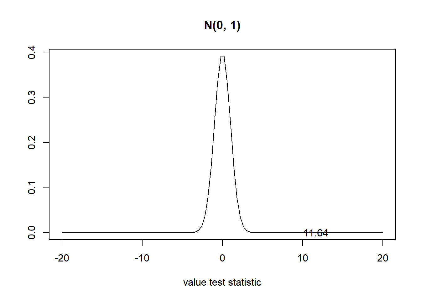
The test statistic is \(z_{obs} = \hat \beta_1/SE(\hat \beta_1) = 11.639\). \(Z \sim N(0, 1)\)
P-value: Probability of observing a test statistic value of 11.639 or more extreme (in both directions) in the null distribution.
\(P(Z > |z_{\mbox{obs}}|)\)
z <-11.6392*(1-pnorm(z))
[1] 0
p-value < 0.05. Reject the null hypothesis \(H_0\). At the significance level 5%, the data provide sufficient evidence that the time has an effect on the number of deaths due to AIDS in Australia
Goodness of fit
\(H_0\): The proposed model fits as well as the saturated model versus
\(H_1\): The saturated model fits better than the proposed model
Choose significance level \(\alpha = 0.05\) so the probability of incorrectly rejecting the null when it is true is 5%.
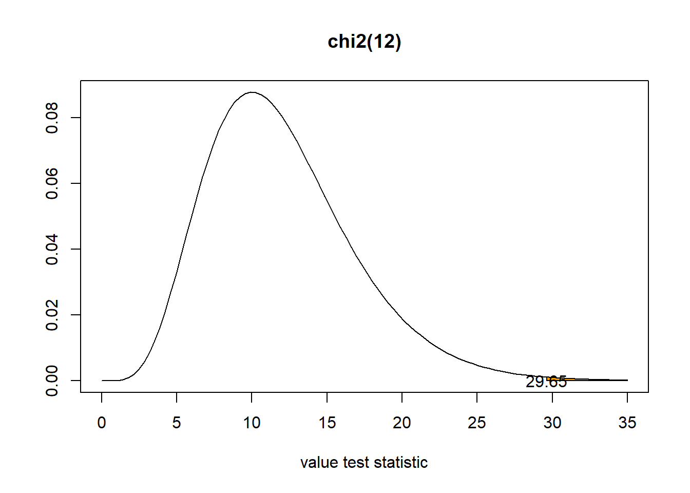
Test statistic: \(D^*\) = 2 (l_s - l_m) \(\sim \chi^2_{df}\) with df difference in the number of parameters = 14-2 = 12
For Poisson deviance and scaled deviance are the same (\(\phi\) = 1)
Under \(H_0\) (proposed model fits as well as the saturated model) the deviance is expected to be small.
p-value: \(P(\chi^2 > 29.654)\) Probability of observing a test statistic value of 29.654 or more extreme in the null distribution.
p-value < 0.05. Reject the null hypothesis \(H_0\). This indicates that the saturated model fits the data significantly better than the model only including time. This residual deviance is indicating lack of model fit for the model only including time to predict death due to AIDS in Australia.
z <-29.654df <-121-pchisq(z, df)
[1] 0.003147356
41.2 GLM Binomial
The following R output reports the result of an experiment for a pesticide which attempted to kill beetles. Beetles were exposed to gaseous carbon disulphide at various concentrations (in mg/L) for five hours and the number of beetles killed were noted.
Call:glm(formula =cbind(Killed, Survived) ~ Dose, family = binomial)>summary(modl)Coefficients: Estimate Std. Error z value Pr(>|z|)(Intercept) -14.823001.28959-11.49<2e-16***Dose 0.249420.0213911.66<2e-16***Null deviance:284.2024 on 7 degrees of freedomResidual deviance:7.3849 on 6 degrees of freedom>vcov(modl) (Intercept) Dose(Intercept) 1.66302995-0.0274363845Dose -0.027436380.0004573762
Write down the fitted model.
Perform a hypothesis test to determine the significance of Dose. You need to state the hypothesis, state the calculated test statistic, state the reference distribution under the null hypothesis, set a decision rule and state the conclusion.
Estimate the odds ratio as well as its significance when Dose increases 4 units. Interpret the odds ratio.
Provide the 95% confidence interval for the probability of killing when the value of Dose equals 62.
GLM Binomial. Solutions
Let \(Y_i\) be the number of beetles killed, \(n_i\) be the total number of beetles, and \(x_i\) the corresponding dose value for each observation \(i\). The fitted model is \[Y_i \sim Bin(n_i, \pi(x_i)),\]\[\mbox{logit}(\pi(x_i)) = \log \left(\frac{\pi(x_i)}{1-\pi(x_i)} \right)= -14.823 + 0.24942x_i\]
We test \(H_0: \beta_1 = 0\) versus \(H_1: \beta_1 \neq 0\).
The test statistic is \(\hat \beta_1/SE(\hat \beta_1) = 0.24942/0.02139=11.66\).
The test statistic distribution under the null hypothesis is N(0,1).
The p-value based on N(0,1) distribution is less than \(0.05\). Therefore, we reject the null hypothesis, Dose is significant.
The interpretation is the odds for beetle to be killed increases 171% if the Dose increases 4 units.
Let \(\eta\) be the value of the linear component when Dose equals to 62. Then, \[\hat \eta = \boldsymbol{x}' \boldsymbol{\hat \beta} = \boldsymbol{x}' (\hat \beta_0, \hat \beta_1)' = (1, 62) (\hat \beta_0, \hat \beta_1)' = -14.823 + 0.24942 \times 62 = 0.6410\]
Then, the 95% confidence interval for \(\eta\) is \[0.6410 \pm 1.96 \sqrt{0.019145} = (0.3699, 0.9121)\] Therefore, the 95% confidence interval for the probability of killing is \[\left(\frac{e^{0.3699}}{1+e^{0.3699}} , \frac{e^{0.9121}}{1+e^{0.9121}} \right) = (0.5914, 0.7134)\]