1 Getting started
1.1 The R ecosystem
1.2 Installing R and RStudio
R (https://www.r-project.org) is a free, open source, software environment for statistical computing and graphics with many excellent packages for importing and manipulating data, statistical modeling, and visualization. R can be downloaded and installed from CRAN (the Comprehensive R Archive Network) (https://cran.rstudio.com). It is recommended to run R using the integrated development environment (IDE) called RStudio. RStudio allows to interact with R more readily and can be freely downloaded from https://www.rstudio.com/products/rstudio/download.
To install R, go to the home website of R www.r-project.org and
- click download CRAN in the left bar
- choose a download site
- choose operation system
- click base
- choose Download R and choose default answers for all questions
To install IDE RStudio, go to www.rstudio.com and
- under Download RStudio, click Download
- below RStudio Desktop (free), click Download
- click the version for your operating system
- download the .exe file and run it and choose default answers for all questions
1.3 RStudio layout
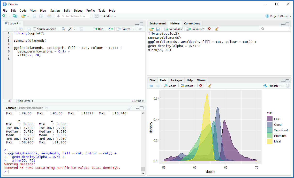
Figure below shows a snapshot of an RStudio IDE with the following four panes:
- Code editor (top-left): This pane is where we create and view the R script files with our work.
- Console (bottom-left): Here we see the execution and the output of the R code. We can execute R code from the code editor or directly enter R commands in the console pane.
- Environment/History (top-right): This pane contains the ‘Environment’ tab with datasets, variables, and other R objects created, and the ‘History’ tab with a history of the previous R commands executed. This pane may also contain other tabs such as ‘Git’ for version control.
- Files/Plots/Packages/Help (bottom-right): Here we can see the files in our working directory (‘Files’ tab), and the graphs generated (‘Plots’ tab). This pane also contains other tabs such as ‘Packages’ and ‘Help’.
2 Modes of interacting with R
Typing commands in the R console
Writing code in script files
- copy-paste commands to the console
- Shortcut to run current line/selection: Ctrl+Enter (Windows), Command+Enter (MacOS)
- Shortcut to run entire script file: Ctrl+Shift+Enter (Windows), Command+Shift+Enter (MacOS)
- read in and execute all commands at once with
source()
2.1 R as calculator
Type the equation in the command window after the >
symbol.
10^2 + 36## [1] 136# Variable assignment
x <- 5+5
x## [1] 10If we use brackets and forget to add the closing bracket, the
> on the command line changes into a +. The
+ can also mean that R is still busy with some heavy
computation. If we want R to quit what it was doing and give back the
>, press ESC.
2.2 Scripts
We can store your commands in scripts. These scripts have file names
with the extension .R. We can open an editor window to edit
these files by clicking File and New or Open file…
We can run the whole script with the console command source, so
e.g. for the script in the file foo.R
source("foo.R")2.4 Working directory
The working directory is the folder on our computer in which we are currently working.
# returns path for the current working directory
getwd()

# set the working directory to a specified directory
setwd("path/of/directory")
Within RStudio we can also go to Session - Set working directory - Choose directory.
2.5 Packages
With the standard installation of R, most common packages are installed. If we need additional functionality, we can also install R packages. The Comprehensive R Archive Network (CRAN) is the main repository for R packages.
To install a package from CRAN we type:
install.packages("packagename")To attach a package to start using it we need to type:
library(packagename)We can see a list of all installed packages in the Packages tab of
RStudio, or by typing installed.packages() or
library().
ls() list objects in the environment. They can also be
seen in the Environment tab of RStudio
data() lists all datasets
rm(x, mx) remove objects
rm(list = ls()) removes all objects from R’s memory
2.6 Getting help
We can get help on specific functions by typing
?functionname or help(functionname)
??functionname searches the function in the
Comprehensive R Archive Network (CRAN) and provides the name of the
package that contains the function
help.start() calls an HTML-based global help
We can also search our question in Google or Stack Overflow (https://stackoverflow.com/)
2.7 System and packages information
System and user information can be retrieved with
Sys.info()Version information about R, the operating system and attached packages
sessionInfo()Package version
packageVersion("sf")3 Data types
3.1 Numbers
Vector of numbers
# vector consisting of 1, 5, and 10
# c() is the 'combine' function
c(1, 5, 10)
## [1] 1 5 10# vector of integers between 1 and 10
1:10 ## [1] 1 2 3 4 5 6 7 8 9 10# assign vector of integers between 1 and 10 to variable x
x <- 1:10
x## [1] 1 2 3 4 5 6 7 8 9 10Regular sequences
# sequence of numbers from 1 to 21 by increments of 2
seq(from = 1, to = 21, by = 2)
## [1] 1 3 5 7 9 11 13 15 17 19 21# sequence of numbers from 1 to 31 with 3 equal incremented numbers
seq(1, 31, length.out = 3) ## [1] 1 16 31Repeated sequences
# replicates x a specified number of times
rep(x = 1:4, times = 2)
## [1] 1 2 3 4 1 2 3 4# each element of x is repeated each times
rep(x = 1:4, each = 2) ## [1] 1 1 2 2 3 3 4 4Random numbers
n <- 10

# generate n random numbers between the default values of 0 and 1
runif(n)
## [1] 0.80825190 0.86440488 0.83792299 0.63020129 0.77438091 0.69731244
## [7] 0.04682129 0.79331743 0.35917790 0.39893421# generate n random numbers between 0 and 25
runif(n, min = 0, max = 25) ## [1] 2.557973 19.409298 16.673220 8.037745 22.873311 23.103512 18.655786
## [8] 23.798240 12.469154 13.033757# generate n random numbers between 0 and 25 (with replacement)
sample(0:25, n, replace = TRUE) ## [1] 10 5 13 10 2 3 10 8 17 3# generate n random numbers between 0 and 25 (without replacement)
sample(0:25, n, replace = FALSE) ## [1] 13 0 12 15 2 5 24 18 19 14Rounding numeric values
x <- c(1, 1.35, 1.7, 2.05, 2.4, 2.75, 3.1, 3.45, 3.8, 4.15, 4.5, 4.85, 5.2, 5.55, 5.9)

# Round to the nearest integer
round(x)
## [1] 1 1 2 2 2 3 3 3 4 4 4 5 5 6 6# Round up
ceiling(x)## [1] 1 2 2 3 3 3 4 4 4 5 5 5 6 6 6# Round down
floor(x)## [1] 1 1 1 2 2 2 3 3 3 4 4 4 5 5 5# Round to a specified decimal
round(x, digits = 1)## [1] 1.0 1.4 1.7 2.0 2.4 2.8 3.1 3.5 3.8 4.2 4.5 4.8 5.2 5.6 5.9Counting elements
length(1:10)## [1] 10Sort a vector
sort(10:1)## [1] 1 2 3 4 5 6 7 8 9 10Unique elements
x <- c(1:3, 2:5)

# which elements are duplicated
duplicated(x)
## [1] FALSE FALSE FALSE TRUE TRUE FALSE FALSE# unique elements (duplicated deleted)
unique(x)## [1] 1 2 3 4 5x[!duplicated(x)]## [1] 1 2 3 4 53.2 Characters
Character strings need to be in quotation marks and can have spaces
a <- "learning to create"    # create string a
b <- "character strings"     # create string b
paste() to concatenate strings
# paste together strings a and b
paste(a, b)
## [1] "learning to create character strings"# paste character and number (converts numbers to character class)
paste("The variable x is equal to", pi) ## [1] "The variable x is equal to 3.14159265358979"# paste multiple strings with a separating character
paste("a", "b", "c", sep = "-") ## [1] "a-b-c"# use paste0() to paste without spaces between characters
paste0("a", "b", "c", "R") ## [1] "abcR"# paste objects with different lengths
paste("R", 1:5, sep = " v1.")## [1] "R v1.1" "R v1.2" "R v1.3" "R v1.4" "R v1.5"Case conversion
x <- "Learning To MANIPULATE strinGS in R"

tolower(x)
## [1] "learning to manipulate strings in r"toupper(x)## [1] "LEARNING TO MANIPULATE STRINGS IN R"Extract or replace substrings in a character vector
alphabet <- paste(LETTERS, collapse = "")

# extract 18-24th characters in string
substr(alphabet, start = 18, stop = 24)
## [1] "RSTUVWX"# replace 19st-24th characters with `R`
substr(alphabet, start = 19, stop = 24) <- "RRRRRR"
alphabet## [1] "ABCDEFGHIJKLMNOPQRRRRRRRYZ"Split string x into substrings according to a substring
split within them
strsplit(x = "aa-bb", split = "-")## [[1]]
## [1] "aa" "bb"3.3 Logicals
Comparing numeric values
x <- 9
y <- 10

x < y     # is x less than y
## [1] TRUEx > y # is x greater than y## [1] FALSEx <= y # is x less than or equal to y## [1] TRUEx >= y # is x greater than or equal to y## [1] FALSEx == y # is x equal to y## [1] FALSEx != y # is x not equal to y## [1] TRUEComparing vector of several elements with a value results in a logical vector
x <- c(5, 14, 10, 22)
x > 13
## [1] FALSE TRUE FALSE TRUE%in% for group membership
3 %in% 1:10## [1] TRUELogical vectors used in ordinary arithmetic are coerced into numeric vectors, FALSE becoming 0 and TRUE becoming 1
x <- c(5, 14, 10, 22)

# how many elements in x are greater than 13?
sum(x > 13)
## [1] 2Position of the vector equal to a number
which(3 == 1:10)## [1] 33.4 Factors
Factors are used to represent categorical data and can be unordered or ordered.
Creating a factor string
gender <- factor(c("male", "female", "female", "male", "female"))
gender
## [1] male female female male female
## Levels: female maleclass(gender)## [1] "factor"levels(gender)## [1] "female" "male"summary(gender)## female male
## 3 2Convert from characters to factors
group <- c("Group1", "Group2", "Group2", "Group1", "Group1")
str(group)
## chr [1:5] "Group1" "Group2" "Group2" "Group1" "Group1"as.factor(group)## [1] Group1 Group2 Group2 Group1 Group1
## Levels: Group1 Group2Ordering levels
# when not specified, the default puts order as alphabetical
gender <- factor(c("male", "female", "female", "male", "female"))
gender
## [1] male female female male female
## Levels: female male# specifying order
gender <- factor(c("male", "female", "female", "male", "female"),
levels = c("male", "female"))
gender## [1] male female female male female
## Levels: male femaleDrop levels
gender <- gender[gender != "male"]

# lets say we have no observations in one level
summary(gender)
## male female
## 0 3# we can drop that level if desired
droplevels(gender)## [1] female female female
## Levels: female3.5 Dates
Getting current date and time
Sys.timezone()## [1] "Asia/Riyadh"Sys.Date()## [1] "2023-03-16"Sys.time()## [1] "2023-03-16 12:23:01 +03"Converting strings to dates using as.Date(). Default
date format is YYYY-MM-DD. For a complete list of
formatting code options type ?strftime
x <- c("2015-07-01", "2015-08-01", "2015-09-01")
as.Date(x)
## [1] "2015-07-01" "2015-08-01" "2015-09-01"y <- c("07/01/2015", "07/01/2015", "07/01/2015")
as.Date(y, format = "%m/%d/%Y")## [1] "2015-07-01" "2015-07-01" "2015-07-01"Creating date sequences
seq(as.Date("2010-1-1"), as.Date("2015-1-1"), by = "years")## [1] "2010-01-01" "2011-01-01" "2012-01-01" "2013-01-01" "2014-01-01"
## [6] "2015-01-01"seq(as.Date('2015-09-15'), as.Date('2015-09-30'), by = "2 days")## [1] "2015-09-15" "2015-09-17" "2015-09-19" "2015-09-21" "2015-09-23"
## [6] "2015-09-25" "2015-09-27" "2015-09-29"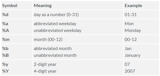
4 Data structures
4.1 Vectors
The basic structure in R is the vector. A vector is a sequence of data elements of the same basic type: numeric, character, logical, factors, or dates.
Creating a vector using :, c(),
seq() or rep()
# integer vector
w <- 8:17
w
## [1] 8 9 10 11 12 13 14 15 16 17# numbers with decimals vector
x <- c(0.5, 0.6, 0.2)
x## [1] 0.5 0.6 0.2# logical vector
y <- c(TRUE, FALSE, FALSE)
y## [1] TRUE FALSE FALSE# Character vector
z <- c("a", "b", "c")
z## [1] "a" "b" "c"Coercing vectors. All elements of a vector must be of the same type. When attempting to combine different types of elements (i.e. character and numeric) they will be coerced to one of the types.
# numerics are turned to characters
str(c("a", "b", "c", 1, 2, 3))
## chr [1:6] "a" "b" "c" "1" "2" "3"# logicals are turned to numerics...
str(c(1, 2, 3, TRUE, FALSE))## num [1:5] 1 2 3 1 0# or characters
str(c("A", "B", "C", TRUE, FALSE))## chr [1:5] "A" "B" "C" "TRUE" "FALSE"Often it is best to explicitly coerce with
as.character(), as.double(),
as.integer(), or as.logical().
class(state.region)## [1] "factor"state.region2 <- as.character(state.region)
class(state.region2)## [1] "character"Adding additional elements to a pre-existing vector
v1 <- 8:17

c(v1, 18:22)
## [1] 8 9 10 11 12 13 14 15 16 17 18 19 20 21 22Subsetting vectors
Subsetting with positive integers
v1## [1] 8 9 10 11 12 13 14 15 16 17v1[2]## [1] 9v1[2:4]## [1] 9 10 11v1[c(2, 4, 6, 8)]## [1] 9 11 13 15# note that we can duplicate index positions
v1[c(2, 2, 4)]## [1] 9 9 11Subsetting with negative integers will omit the elements at the specified positions
v1[-1]## [1] 9 10 11 12 13 14 15 16 17v1[-c(2, 4, 6, 8)]## [1] 8 10 12 14 16 17Subsetting with logical values will select the elements where the corresponding logical value is TRUE
v1[c(TRUE, FALSE, TRUE, FALSE, TRUE, TRUE, TRUE, FALSE, FALSE, TRUE)]## [1] 8 10 12 13 14 17v1[v1 < 12]## [1] 8 9 10 11v1[v1 < 12 | v1 > 15]## [1] 8 9 10 11 16 174.2 Lists
A list is an R structure that allows us to combine elements of different types
Creating Lists
l <- list(1:3, "a", c(TRUE, FALSE, TRUE), c(2.5, 4.2))
str(l)
## List of 4
## $ : int [1:3] 1 2 3
## $ : chr "a"
## $ : logi [1:3] TRUE FALSE TRUE
## $ : num [1:2] 2.5 4.2Adding additional list components to a list
We can add a new list component by utilizing the $ sign
and naming the new item
l1 <- list(1:3, "a", c(TRUE, FALSE, TRUE))
str(l1)
## List of 3
## $ : int [1:3] 1 2 3
## $ : chr "a"
## $ : logi [1:3] TRUE FALSE TRUEl1$item4 <- "new list item"
str(l1)## List of 4
## $ : int [1:3] 1 2 3
## $ : chr "a"
## $ : logi [1:3] TRUE FALSE TRUE
## $ item4: chr "new list item"To add additional values to a list item, we need to subset that
specific list item and then we can use the c() function to
add the additional elements to that list item
l1[[1]] <- c(l1[[1]], 4:6)
str(l1)
## List of 4
## $ : int [1:6] 1 2 3 4 5 6
## $ : chr "a"
## $ : logi [1:3] TRUE FALSE TRUE
## $ item4: chr "new list item"l1[[2]] <- c(l1[[2]], c("dding", "to a", "list"))
str(l1)## List of 4
## $ : int [1:6] 1 2 3 4 5 6
## $ : chr [1:4] "a" "dding" "to a" "list"
## $ : logi [1:3] TRUE FALSE TRUE
## $ item4: chr "new list item"Adding names to a pre-existing list
names(l1) <- c("item1", "item2", "item3")Subsetting lists
Subset list and preserve output as a list
# extract first list item
l1[1]
## $item1
## [1] 1 2 3 4 5 6l1["item1"]## $item1
## [1] 1 2 3 4 5 6# extract multiple list items
l1[c(1, 3)]## $item1
## [1] 1 2 3 4 5 6
##
## $item3
## [1] TRUE FALSE TRUEl1[c("item1", "item3")]## $item1
## [1] 1 2 3 4 5 6
##
## $item3
## [1] TRUE FALSE TRUESubset list and simplify output
# extract first list item and simplify to a vector
l1[[1]]
## [1] 1 2 3 4 5 6l1[["item1"]]## [1] 1 2 3 4 5 6l1$item1## [1] 1 2 3 4 5 6Extract individual elements out of a specific list item
# extract third element from the second list item
l1[[2]][3]
## [1] "to a"l1[["item2"]][3]## [1] "to a"l1$item2[3]## [1] "to a"4.3 Matrices
A matrix is a collection of data elements arranged in a two-dimensional rectangular layout. In R, the elements that make up a matrix must be of a consistent mode (i.e. all elements must be numeric, or character, etc.).
Creating Matrices. Matrices are constructed column-wise, so entries can be thought of starting in the “upper left” corner and running down the columns.
m1 <- matrix(1:6, nrow = 2, ncol = 3)
m1
## [,1] [,2] [,3]
## [1,] 1 3 5
## [2,] 2 4 6m2 <- matrix(letters[1:6], nrow = 2, ncol = 3)
m2## [,1] [,2] [,3]
## [1,] "a" "c" "e"
## [2,] "b" "d" "f"Matrices can also be created using the column-bind
cbind() and row-bind rbind() functions. The
vectors that are being binded must be of equal length.
v1 <- 1:4
v2 <- 5:8
cbind(v1, v2)
## v1 v2
## [1,] 1 5
## [2,] 2 6
## [3,] 3 7
## [4,] 4 8rbind(v1, v2)## [,1] [,2] [,3] [,4]
## v1 1 2 3 4
## v2 5 6 7 8v3 <- 9:12
cbind(v1, v2, v3)## v1 v2 v3
## [1,] 1 5 9
## [2,] 2 6 10
## [3,] 3 7 11
## [4,] 4 8 12Adding on to matrices
m1 <- cbind(v1, v2)
m1
## v1 v2
## [1,] 1 5
## [2,] 2 6
## [3,] 3 7
## [4,] 4 8# add a new column
cbind(m1, v3)## v1 v2 v3
## [1,] 1 5 9
## [2,] 2 6 10
## [3,] 3 7 11
## [4,] 4 8 12# add a new row
rbind(m1, c(4.1, 8.1))## v1 v2
## [1,] 1.0 5.0
## [2,] 2.0 6.0
## [3,] 3.0 7.0
## [4,] 4.0 8.0
## [5,] 4.1 8.1Adding names
m2 <- matrix(1:12, nrow = 4, ncol = 3)
m2
## [,1] [,2] [,3]
## [1,] 1 5 9
## [2,] 2 6 10
## [3,] 3 7 11
## [4,] 4 8 12# the dimension attribute shows this matrix has 4 rows and 3 columns
attributes(m2)## $dim
## [1] 4 3# add row names as an attribute
rownames(m2) <- c("row1", "row2", "row3", "row4")
m2## [,1] [,2] [,3]
## row1 1 5 9
## row2 2 6 10
## row3 3 7 11
## row4 4 8 12attributes(m2)## $dim
## [1] 4 3
##
## $dimnames
## $dimnames[[1]]
## [1] "row1" "row2" "row3" "row4"
##
## $dimnames[[2]]
## NULL# add column names
colnames(m2) <- c("col1", "col2", "col3")
m2## col1 col2 col3
## row1 1 5 9
## row2 2 6 10
## row3 3 7 11
## row4 4 8 12attributes(m2)## $dim
## [1] 4 3
##
## $dimnames
## $dimnames[[1]]
## [1] "row1" "row2" "row3" "row4"
##
## $dimnames[[2]]
## [1] "col1" "col2" "col3"Subsetting matrices
A generic form of matrix subsetting looks like:
matrix[rows, columns]
# subset for rows 1 and 2 but keep all columns
m2[1:2, ]
## col1 col2 col3
## row1 1 5 9
## row2 2 6 10# subset for columns 1 and 3 but keep all rows
m2[ , c(1, 3)]## col1 col3
## row1 1 9
## row2 2 10
## row3 3 11
## row4 4 12# subset for both rows and columns
m2[1:2, c(1, 3)]## col1 col3
## row1 1 9
## row2 2 10# use a vector to subset
v <- c(1, 2, 4)
m2[v, c(1, 3)]## col1 col3
## row1 1 9
## row2 2 10
## row4 4 12# use names to subset
m2[c("row1", "row3"), ]## col1 col2 col3
## row1 1 5 9
## row3 3 7 11Note that subsetting matrices with the [
operator will simplify the results to the lowest possible dimension. To
avoid this we can introduce the drop = FALSE
argument
# simplifying results in a named vector
m2[, 2]
## row1 row2 row3 row4
## 5 6 7 8# preserving results in a 4x1 matrix
m2[, 2, drop = FALSE]## col2
## row1 5
## row2 6
## row3 7
## row4 84.4 Data frames
A data frame is a list of equal-length vectors. Each element of the list can be thought of as a column and the length of each element of the list is the number of rows. As a result, data frames can store different classes of objects in each column (i.e. numeric, character, factor).
Creating data frames
df <- data.frame(col1 = 1:3,
                 col2 = c("this", "is", "text"),
                 col3 = c(TRUE, FALSE, TRUE),
                 col4 = c(2.5, 4.2, pi))

# structure of a data frame
str(df)
## 'data.frame': 3 obs. of 4 variables:
## $ col1: int 1 2 3
## $ col2: chr "this" "is" "text"
## $ col3: logi TRUE FALSE TRUE
## $ col4: num 2.5 4.2 3.14# number of rows
nrow(df)## [1] 3# number of columns
ncol(df)## [1] 4data.frame() has an argument
stringsAsFactors = default.stringsAsFactors() to specify
whether character columns should be converted to factors. We can turn
this off by setting stringsAsFactors = FALSE
default.stringsAsFactors()## Warning: 'default.stringsAsFactors' is deprecated.
## Use '`stringsAsFactors = FALSE`' instead.
## See help("Deprecated")## [1] FALSEdf <- data.frame(col1 = 1:3,
col2 = c("this", "is", "text"),
col3 = c(TRUE, FALSE, TRUE),
col4 = c(2.5, 4.2, pi),
stringsAsFactors = FALSE)
# note how col2 now is of a character class
str(df)## 'data.frame': 3 obs. of 4 variables:
## $ col1: int 1 2 3
## $ col2: chr "this" "is" "text"
## $ col3: logi TRUE FALSE TRUE
## $ col4: num 2.5 4.2 3.14Converting pre-existing structures to a data frame
v1 <- 1:3
v2 <- c("this", "is", "text")
v3 <- c(TRUE, FALSE, TRUE)

# convert same length vectors to a data frame using data.frame()
data.frame(col1 = v1, col2 = v2, col3 = v3)
# convert a list to a data frame using as.data.frame()
l <- list(item1 = 1:3, item2 = c("this", "is", "text"), item3 = c(2.5, 4.2, 5.1))
as.data.frame(l)# convert a matrix to a data frame using as.data.frame()
m1 <- matrix(1:12, nrow = 4, ncol = 3)
as.data.frame(m1)Adding on to data frames
df# add a new column
v4 <- c("A", "B", "C")
cbind(df, v4)Adding attributes to data frames
rownames(df) <- c("row1", "row2", "row3")
dfattributes(df)## $names
## [1] "col1" "col2" "col3" "col4"
##
## $class
## [1] "data.frame"
##
## $row.names
## [1] "row1" "row2" "row3"Change the existing column names by using colnames() or
names()
# add/change column names with colnames()
colnames(df) <- c("col_1", "col_2", "col_3", "col_4")
df
# add/change column names with names()
names(df) <- c("col.1", "col.2", "col.3", "col.4")
dfSubsetting data frames
# subsetting by row numbers
df[2:3, ]
# subsetting by row names
df[c("row2", "row3"), ]# subsetting columns like a list
df[c("col.2", "col.4")]# subsetting columns like a matrix
df[, c("col.2", "col.4")]# subset for both rows and columns
df[1:2, c(1, 3)]# use a vector to subset
v <- c(1, 2, 4)
df[, v]Note that subsetting data frames with the [
operator will simplify the results to the lowest possible dimension. To
avoid this we can set drop = FALSE.
# simplifying results in a named vector
df[, 2]
## [1] "this" "is" "text"# preserving results in a 3x1 data frame
df[, 2, drop = FALSE]Subset data frames based on conditional statements
head(mtcars)# using brackets
mtcars[mtcars$mpg > 20, ]# using the subset function
subset(mtcars, mpg > 20)# using brackets
mtcars[mtcars$mpg > 20 & mtcars$cyl == 6, ]# using the subset function
subset(mtcars, mpg > 20 & cyl == 6)# using brackets
mtcars[mtcars$mpg > 20 & mtcars$cyl == 6, c("mpg", "cyl", "wt")]# using the subset function
subset(mtcars, mpg > 20 & cyl == 6, c("mpg", "cyl", "wt"))4.5 NAs
A common task in data analysis is dealing with missing values. In R, missing values are often represented by NA (NA = not available)
Identifying missing values using is.na()
x <- c(1:4, NA, 6:7, NA)
is.na(x)
## [1] FALSE FALSE FALSE FALSE TRUE FALSE FALSE TRUEdf <- data.frame(col1 = c(1:3, NA),
col2 = c("this", NA,"is", "text"),
col3 = c(TRUE, FALSE, TRUE, TRUE),
col4 = c(2.5, 4.2, 3.2, NA),
stringsAsFactors = FALSE)
is.na(df)## col1 col2 col3 col4
## [1,] FALSE FALSE FALSE FALSE
## [2,] FALSE TRUE FALSE FALSE
## [3,] FALSE FALSE FALSE FALSE
## [4,] TRUE FALSE FALSE TRUEis.na(df$col4)## [1] FALSE FALSE FALSE TRUELocation of NAs
# identify location of NAs in vector
which(is.na(x))
## [1] 5 8Number of NAs
# identify count of NAs in data frame
sum(is.na(df))
## [1] 3Total missing values in each column
colSums(is.na(df))## col1 col2 col3 col4
## 1 1 0 1Recode missing values
# vector with missing data
x <- c(1:4, NA, 6:7, NA)
# recode missing values with the mean
x[is.na(x)] <- mean(x, na.rm = TRUE)
round(x, 2)
## [1] 1.00 2.00 3.00 4.00 3.83 6.00 7.00 3.83# data frame that codes missing values as 99
df <- data.frame(col1 = c(1:3, 99), col2 = c(2.5, 4.2, 99, 3.2))
# change 99s to NAs
df[df == 99] <- NA
df# data frame with missing data
df <- data.frame(col1 = c(1:3, NA),
col2 = c("this", NA,"is", "text"),
col3 = c(TRUE, FALSE, TRUE, TRUE),
col4 = c(2.5, 4.2, 3.2, NA),
stringsAsFactors = FALSE)
df$col4[is.na(df$col4)] <- mean(df$col4, na.rm = TRUE)
dfExclude missing values
# A vector with missing values
x <- c(1:4, NA, 6:7, NA)

# including NA values produces an NA output
mean(x)
## [1] NA# excluding NA values calculates the mathematical operation for all non-missing values
mean(x, na.rm = TRUE)## [1] 3.833333Subset of observations (rows) in our data that contain no missing data
# data frame with missing values
df <- data.frame(col1 = c(1:3, NA),
                 col2 = c("this", NA,"is", "text"),
                 col3 = c(TRUE, FALSE, TRUE, TRUE),
                 col4 = c(2.5, 4.2, 3.2, NA),
                 stringsAsFactors = FALSE)

complete.cases(df)
## [1] TRUE FALSE TRUE FALSE# subset with complete.cases to get the complete rows
df[complete.cases(df), ]# or subset with `!` operator to get the incomplete rows
df[!complete.cases(df), ]# or use na.omit() to get the complete rows
na.omit(df)5 Importing data
Text file formats use delimiters to separate the different elements
in a line, and each line of data is in its own line in the text file. To
import a text file we can use read.table() which is a
multipurpose function in base R for importing data.
read.csv() and read.delim() are special cases
of read.table(). Alternatively, we can use function
read_csv() from the readr package, and
function fread() from the data.table package
which are faster.
variable 1,variable 2,variable 3
10,beer,TRUE
25,wine,TRUE
8,cheese,FALSE
mydata <- read.csv("mydata.csv")
mydata
# this is the same
mydata <- read.table("mydata.csv", sep = ",", header = TRUE, stringsAsFactors = FALSE)# invoke a spreadsheet-style data viewer on a matrix-like R object
View(mydata)
str(mydata)To import Excel files, we can simply export the Excel file as a CSV
file and then import into R using read.csv(). We can also
use the functions in the readxl package.
With the file.choose() function we can simply choose the
file we want to open by clicking some buttons.
d <- read.csv(file.choose())The foreign package can be used to read data from other
programming languages (e.g., .sav for SPSS data).
Importing R object files
load("mydata.RData")

load(file = "mydata.rda")

readRDS("mydata.rds")
We can use attach() to keep the dataset as the current
or working dataset. By doing that we will not need to keep using the
$ sign to point to the data set, we can just call the
variables in the dataset by name. For example:
# mean(Temp)
mean(airquality$Temp)
## [1] 77.88235attach(airquality)
mean(Temp)## [1] 77.88235We should never attach two datasets that have the same variable names as this could lead to confusion.
6 Exporting data
write.table() is the multipurpose function in base R for
exporting data. The functions write.csv() and
write.delim() are special cases of
write.table() in which the defaults have been adjusted for
efficiency. We can also use write_csv() from the
readr package.
df <- data.frame(var1 = c(10, 25, 8),
                 var2 = c("beer", "wine", "cheese"),
                 var3 = c(TRUE, TRUE, FALSE),
                 row.names = c("billy", "bob", "thornton"))

# write to a csv file
write.csv(df, file = "export_csv")

# write to a csv and save in a different directory
write.csv(df, file = "folder/subfolder/subsubfolder/export_csv")

# write to a csv file with added arguments
write.csv(df, file = "export_csv", row.names = FALSE, na = "MISSING!")
Exporting R object files
Sometimes we may need to save data or other R objects outside of our
workspace. There are three primary ways that people tend to save R
data/objects: as .RData, .rda, or
.rds files.
.rda is just short for .RData, therefore,
these file extensions represent the same underlying object type. We use
the .rda or .RData file types when we want to
save several, or all, objects and functions that exist in our global
environment.
On the other hand, if we only want to save a single R object such as
a data frame, function, or statistical model results its best to use
.rds file type. We can use .rda or
.RData to save a single object but the benefit of
.rds is it only saves a representation of the object and
not the name whereas .rda and .RData save the
both the object and its name. As a result, with .rds the
saved object can be loaded into a named object within R that is
different from the name it had when originally saved.
# save() can be used to save multiple objects in our global environment,
# in this case we save two objects to a .RData file
x <- stats::runif(20)
y <- list(a = 1, b = TRUE, c = "oops")
save(x, y, file = "xy.RData")

# save.image() is just a short-cut for 'save my current workspace',
# i.e. all objects in our global environment
save.image()

# save a single object to file
saveRDS(x, "x.rds")

# restore it under a different name
x2 <- readRDS("x.rds")
identical(x, x2)
7 Graphics
plot() is the generic function for plotting R
objects.
x <- rnorm(100)
plot(x)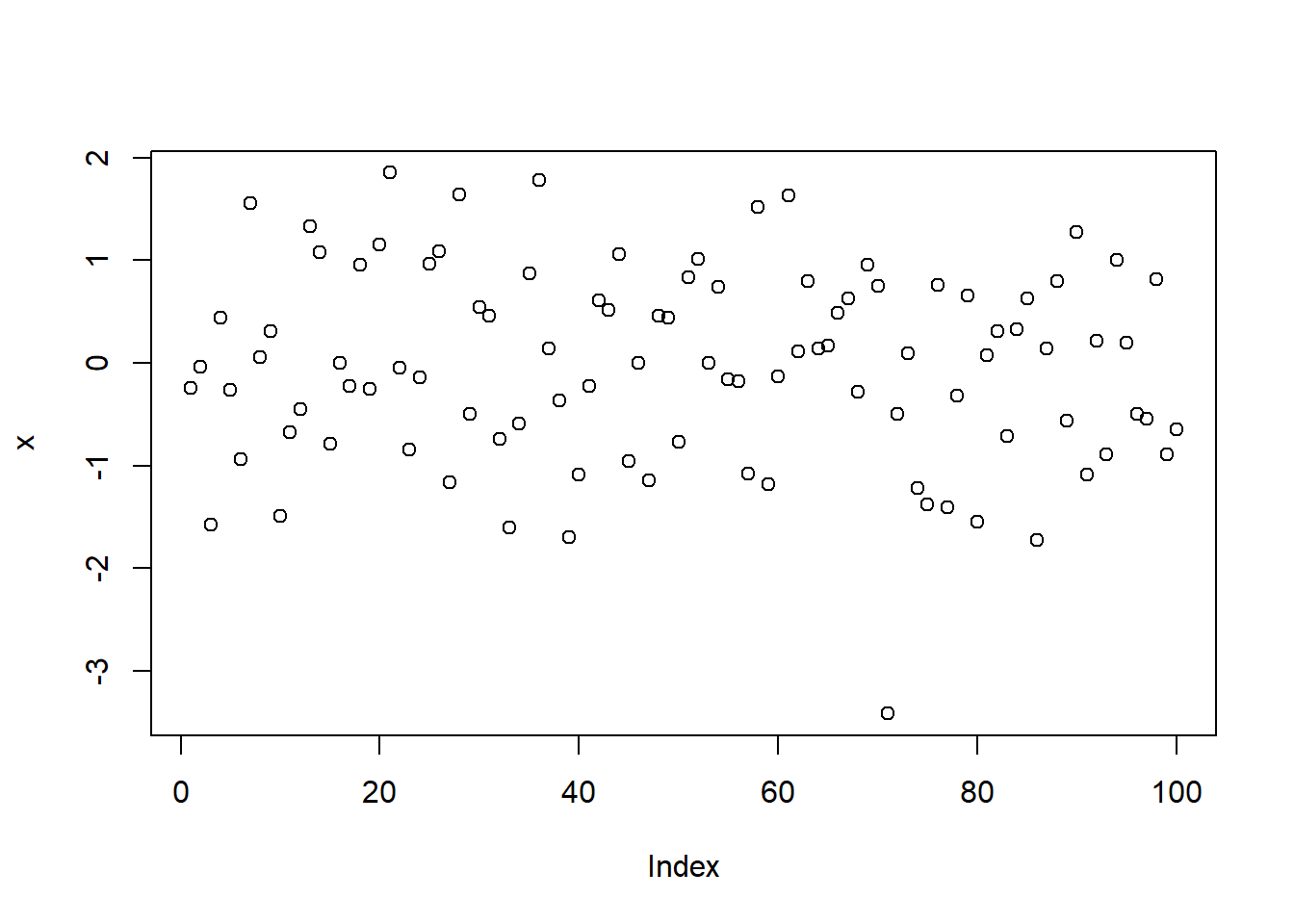
plot(rnorm(100), type = "l", col = "red")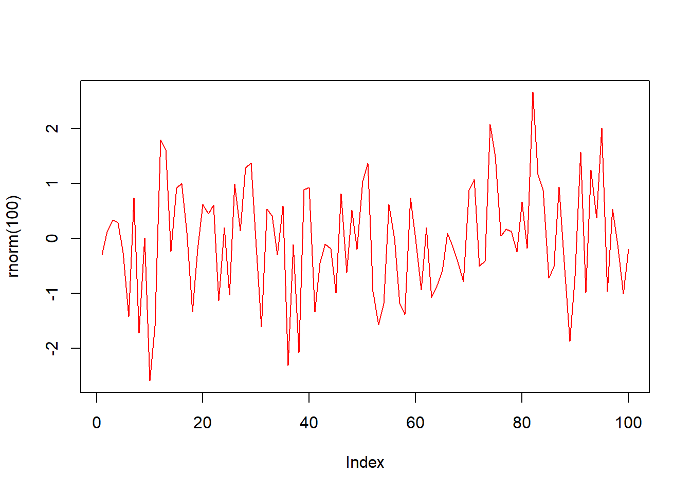
hist() computes histograms
hist(rnorm(100))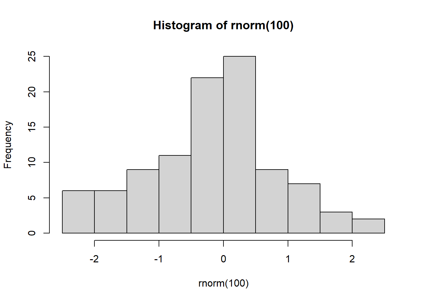
d <- data.frame(a = rnorm(100), b = rnorm(100), c = rnorm(100))

plot(d$a, type = "l", ylim = range(d), lwd = 3, col = "red")
lines(d$b, type = "s", lwd = 2, col = "green")
points(d$c, pch = 20, cex = 4, col = "blue")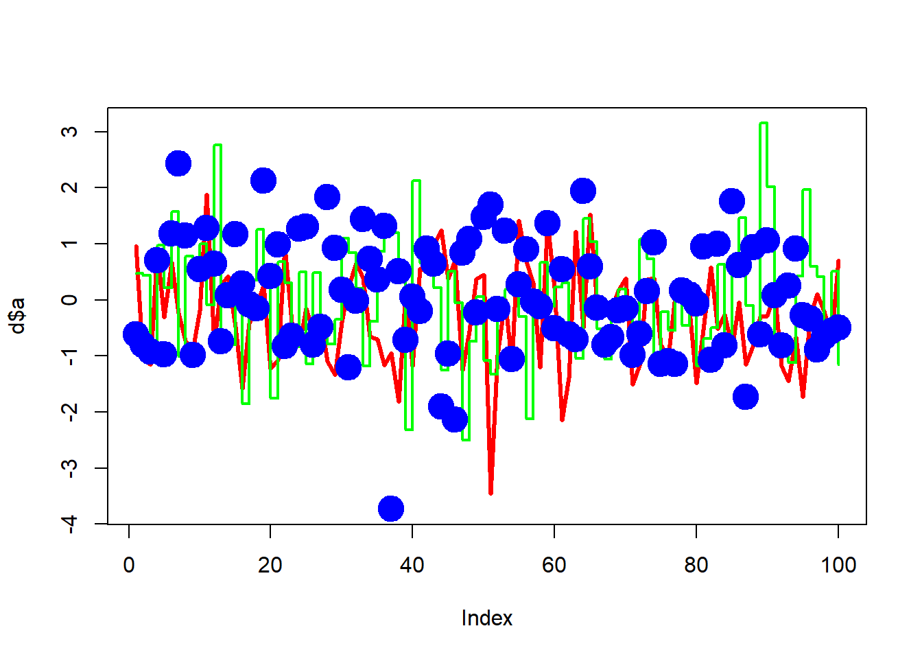
Type ?plot.default to know more about the arguments of
the function.
We will also see the package ggplot2 for plotting data:
https://ggplot2.tidyverse.org/
8 Functions
Functions allows us to automate common tasks. Key steps to creating a new function:
- Pick a name for the function
- List the inputs or arguments
- Place the code in body of the function
# Define the function
fnRescale01 <- function(x) {
  rng <- range(x, na.rm = TRUE)
  return((x - rng[1]) / (rng[2] - rng[1]))
}

# Execute the function
x <- c(0, 5, 10)
fnRescale01(x)
The txtProgressBar() and
setTxtProgressBar() functions from the utils
package can be used to show a text progress bar in the R console. This
is useful to show in long computations.
2.3 Comments
Write comments with
#R is case sensitive, so we need to make sure we write capital letters where necessary.