Reproducible reports with R Markdown
1 Reproducible reports and dashboards
2 R Markdown
The package rmarkdown allows us to easily turn our
analyses into fully reproducible documents that can be shared with
others in a variety of formats including HTML and PDF. An R Markdown
document is a text file with extension .Rmd that
intermingles text and R code, and can include narrative text, tables and
visualizations. When the R Markdown document is compiled, the R code is
executed and a report with the output of the R code is created.
Resources to learn R Markdown include book1 and book2. Reference: https://www.rstudio.com/wp-content/uploads/2015/03/rmarkdown-reference.pdf
A new R Markdown document (.Rmd) can be created by
clicking File > New File > R Markdown in RStudio.
From the .Rmd file, a report can be generated using the
Knit button in RStudio or executing
rmarkdown::render("name.Rmd", "output_document"), where
name.Rmd is the name of the .Rmd file, and
"output_document" the type of output (e.g.,
"html_document", "pdf_document"). Note that
Latex is needed to generate PDF documents. The Latex distribution
TinyTeX can be installed with the tinytex package with
tinytex::install_tinytex() REF,
Alternatively, Latex can be installed using these resources.
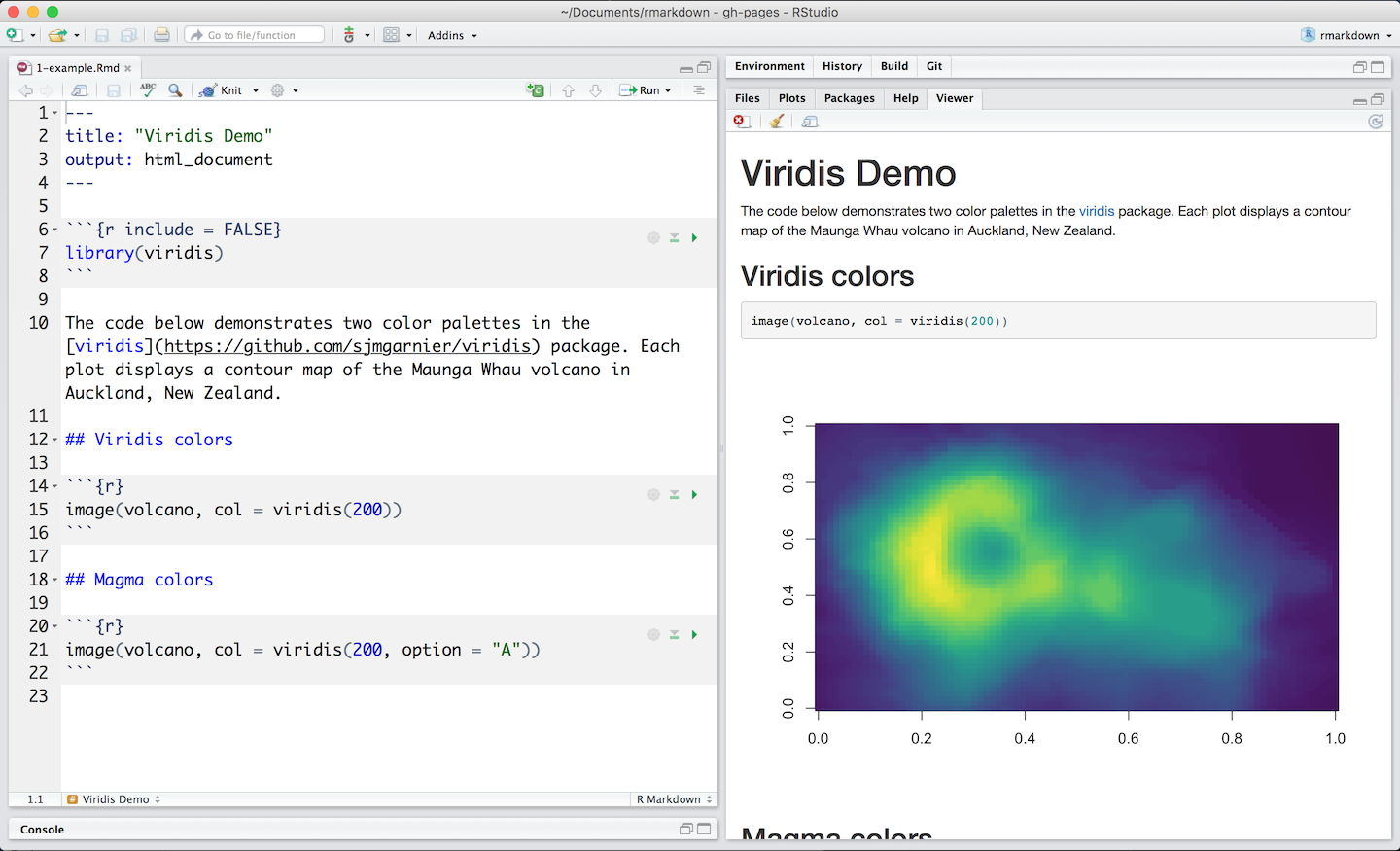
An R Markdown document includes three basic components, namely, a YAML header, Markdown text and R code chunks as follows.
At the beginning of the document, we write a YAML header surrounded
by --- that indicates several options such as title,
author, date and type of output file.
---
title: "Report"
author: "Paula Moraga"
date: 1 July 2023
output: html_document
---
The text is written in Markdown syntax. For example, we can use
asterisks for italic text (*text*) and double asterisks for
bold text (**text**) . We can also include equations in
Latex. See, for example, this equation
editor for examples.
The R code is written within R code chunks which start with three
backticks ```{r} and end with three backticks
```. R code chunks can be specified using several options
like echo=FALSE to hide code and warning=FALSE
to supress warnings.
```{r, warning = FALSE}
# R code to be executed
```
In R chunks, we can include images using
knitr::include_graphics("path/img.png") and tables created
with knitr::kable(). We can also include HTML widgets such as objects
created with leaflet, DT and
dygraphs.
Icons can be included with the fontawesome package. Icons: https://fontawesome.com/v4/icons/. Animated icons: https://emitanaka.org/anicon/
R code chunks can be specified using several options like the following:
echo=FALSEcode will not be shown in the document, but it will run and the output will be displayed in the documenteval=FALSEcode will not run, but it will be shown in the documentinclude=FALSEcode will run, but neither the code nor the output will be included in the documentresults='hide'output will not be shown, but the code will run and will be displayed in the documentcache=TRUEcode chunk is not executed if it has been executed before and nothing in the code chunk has changed since thenerror=FALSE,warning=FALSE,message=FALSEsupress errors, warnings or messages
Example
The code below shows an example of R Markdown document. In the document, the YAML header has the following options:
toc: trueandtoc_float: trueto put a table of contents floating on the leftnumber_sections: trueto number sectionstoc_depth: 2to specify the lowest level of headings to add to the table of contents equal to 2theme: unitedto specify the theme andhighlight: tangoto specify the highlight options. Details about these options can be seen at here.
---
title: "Report"
author: "Paula Moraga"
date: "`r Sys.Date()`"
output:
  html_document:
    toc: true
    toc_float: true
    number_sections: true
    toc_depth: 2
    theme: united
    highlight: tango
---

# First-level header

**Bold text**

[Hyperlink R Markdown](https://rmarkdown.rstudio.com/)

## Second-level header

- unordered item
- unordered item
    1. first item
    2. second item
    3. third item

### Third-level header

```{r, warning=FALSE}
x <- 1:10
y <- 1:10
plot(x, y)
```

$$\int_0^\infty e^{-x^2} dx=\frac{\sqrt{\pi}}{2}$$
2.1 Child documents
https://bookdown.org/yihui/rmarkdown-cookbook/child-document.html
```{r, child = c("child.Rmd")}
```
Exercises
Include the introduction as a child document
2.2 Parameters
https://bookdown.org/yihui/rmarkdown/parameterized-reports.html
Exercises
Include parameter named printcode and use it inside R
chunks to set echo = params$printcode
---
title: My document
output: html_document
params:
  printcode: TRUE
---2.4 Tips for R Markdown
Pimp my RMD: a few tips for R Markdown
Tricks:
https://www.rstudio.com/blog/r-markdown-tips-tricks-1-rstudio-ide/
https://www.rstudio.com/blog/r-markdown-tips-tricks-2-cleaning-up-your-code/
https://www.rstudio.com/blog/r-markdown-tips-and-tricks-3-time-savers/
https://www.rstudio.com/blog/r-markdown-tips-tricks-4-looks-better-works-better/
3 Flexdashboard
The flexdashboard package allows us to create
dashboards on HTML format that contain several related data
visualizations. Examples of dashboards created with
flexdashboard can be seen at the RStudio
website. To create a flexdashboard, we need to write an R Markdown
file with extension .Rmd. The YAML header of the
flexdashaboard document needs to have the option
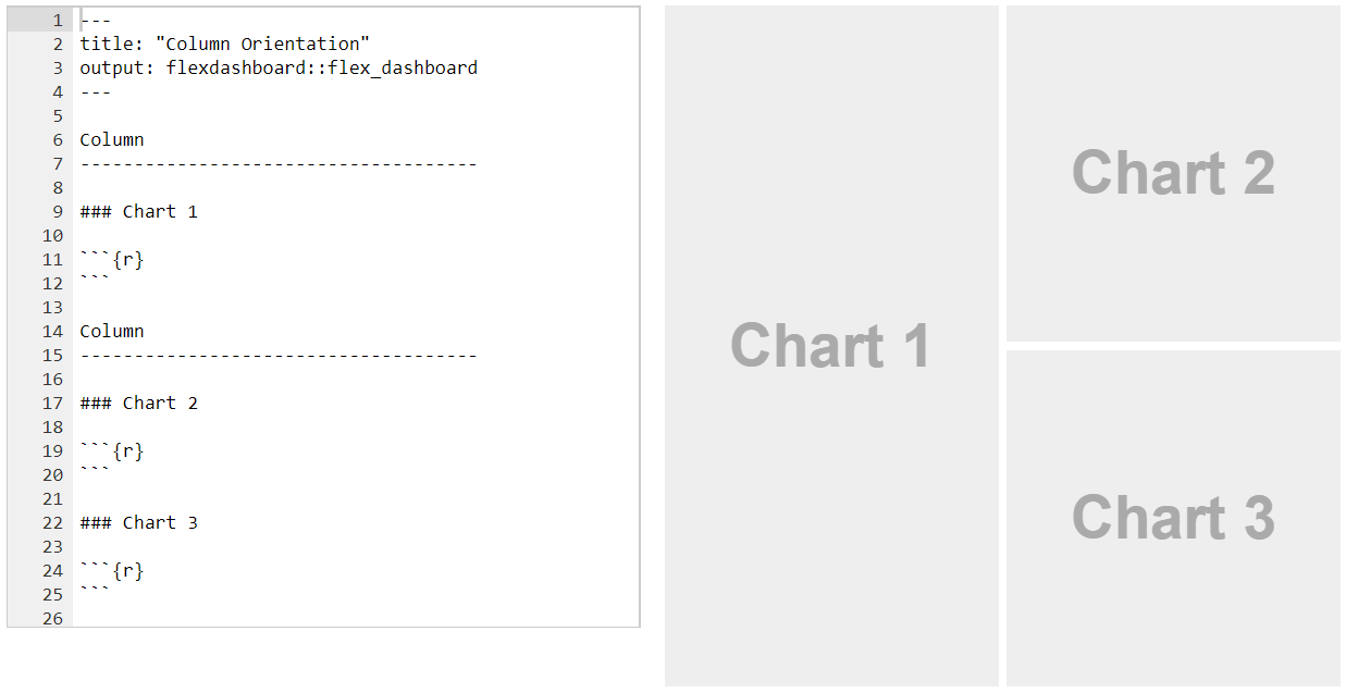
output: flexdashboard::flex_dashboard. Dashboard components
are shown according to a layout that specifies the columns and rows.
Columns are included with --------------, and rows for each
column with ###. Layouts can also be specified row-wise
rather than column-wise by adding orientation: rows in the
YAML. The code below creates a layout with two columns with one and two
components, respectively. Additional layout examples including tabs,
multiple pages and sidebars can be seen at the R
Markdown website.
The R code to create the dashboard’s visualizations is written within R code chunks. Dashboards can contain a wide variety of components including images, tables, equations, and HTML widgets. They can also contain value boxes to display single values with titles and icons, and gauges that display values on a meter within a specified range. Moreover, it is also possible to include navigation bars with links to social services, source code, or other links related to the dashboard.