1 Colors

In R we can specify a color in several ways:

string names (e.g., "blue"). Type colors() to obtain a list of available color names. https://www.nceas.ucsb.edu/sites/default/files/2020-04/colorPaletteCheatsheet.pdf
hex codes (e.g., "#E36D11"). # followed by 6 digits ranging from 0 to F and where first two digits represent redness, second two greenness, and last two blueness. https://htmlcolorcodes.com/
rgb() specifying three numbers between 0 and 1 to get hex code (e.g., rgb(.75, 0, 1) returns “#BF00FF”)

When we map a variable to color or fill, ggplot2 uses the type of variable (i.e., numeric, factor) to choose a color scale.

We can change default by colors using colors from packages such as RColorBrewer or viridis or by manually changing the colors.

RColorBrewer package uses ColorBrewer sequential (e.g., Blues, YlOrRd), diverging (e.g., RdGy, Spectral), or qualitative scale (e.g., Accent, Dark2) colors http://colorbrewer2.org

2 Continuous variables

Default for continuous variables is a color gradient that runs from a blueish-black to light-blue (scale_color_gradient()).

Other possible color scales include scale_color_distiller(), scale_color_fermenter(), scale_color_viridis(), scale_color_gradient(), scale_color_gradient2() and scale_color_gradientn().

library(ggplot2)
ggplot(mtcars, aes(x = wt, y = mpg, color = qsec)) + geom_point()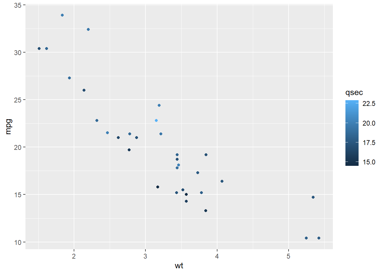

3 Categorical variables

Default for categorical variables is a set of distinct hues evenly spaced around the color wheel (scale_color_hue()).

Other possible color scales include scale_color_brewer() scale_color_viridis() scale_color_grey() and scale_color_manual().

mtcars$cyl <- factor(mtcars$cyl)
ggplot(mtcars, aes(x = wt, y = mpg, color = cyl)) + geom_point()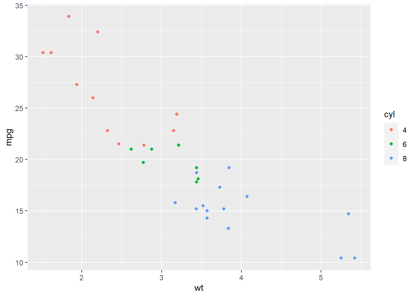

4 Examples

Here we present some examples of color scale functions. There are analogous scale functions for the fill aesthetic.

4.1 Discrete colors

# Single color
ggplot(mtcars, aes(x = wt, y = mpg)) + geom_point(color = "blue")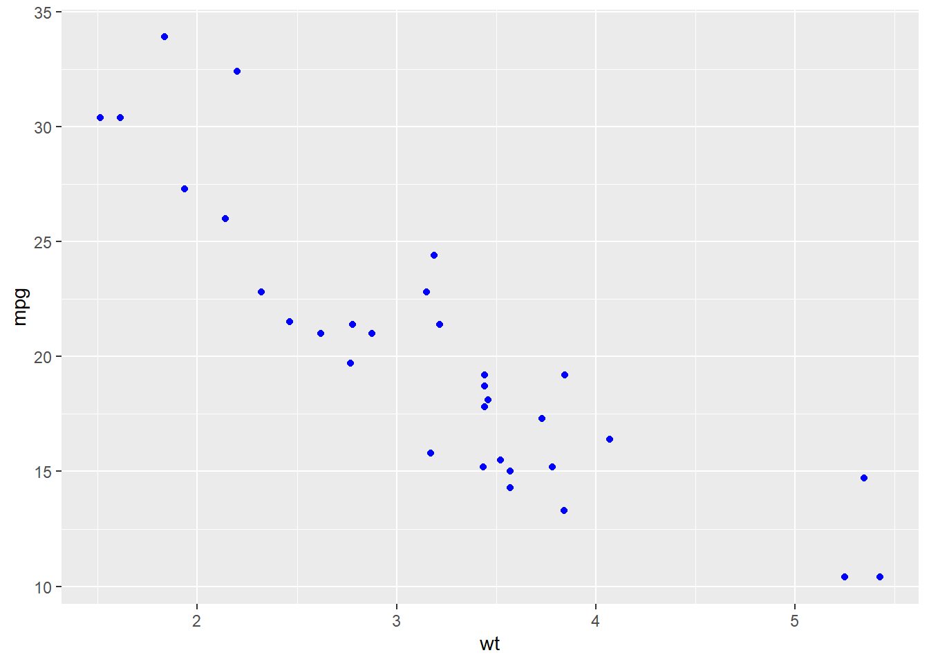

# Color by group (default scale_color_hue())
(g <- ggplot(mtcars, aes(x = wt, y = mpg, color = factor(cyl))) + geom_point())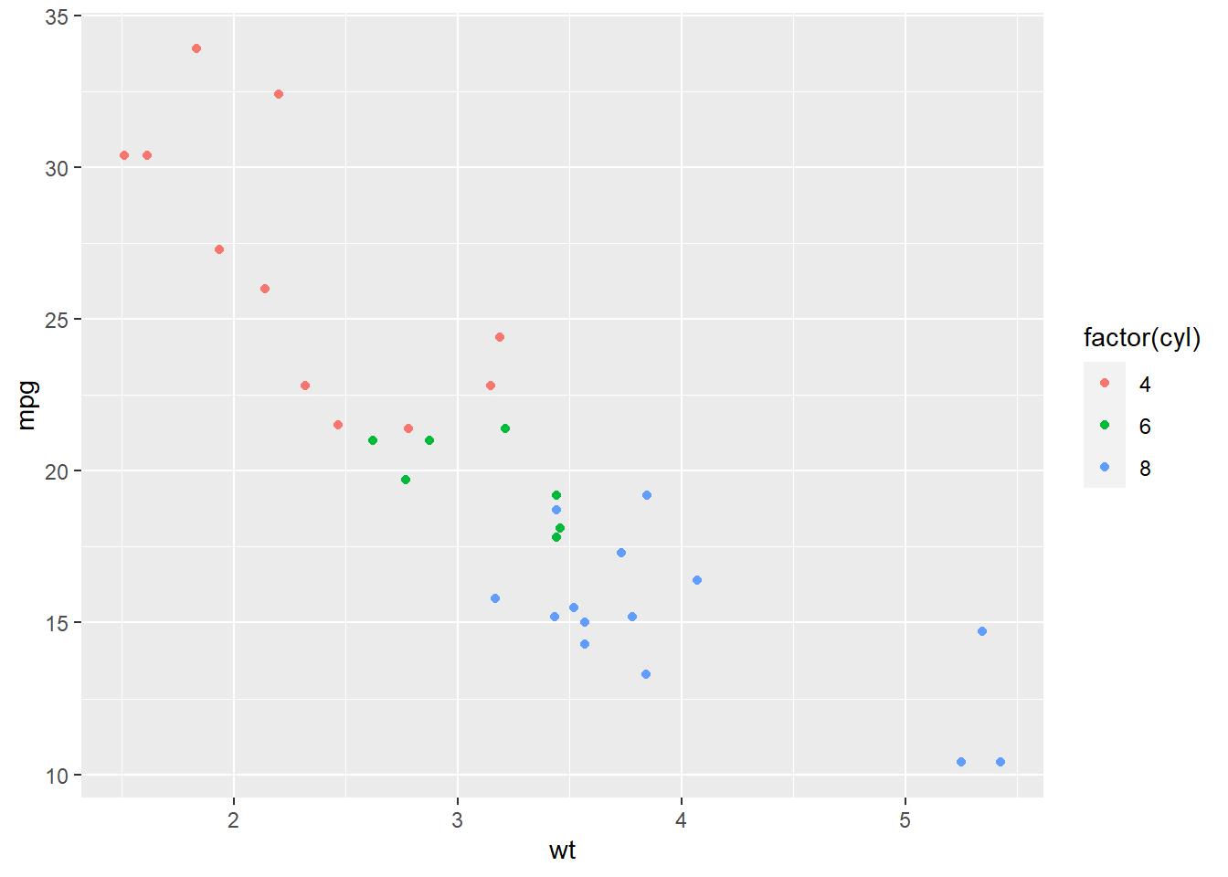

# RColorBrewer palette
library(RColorBrewer)
g + scale_color_brewer(palette = "Dark2")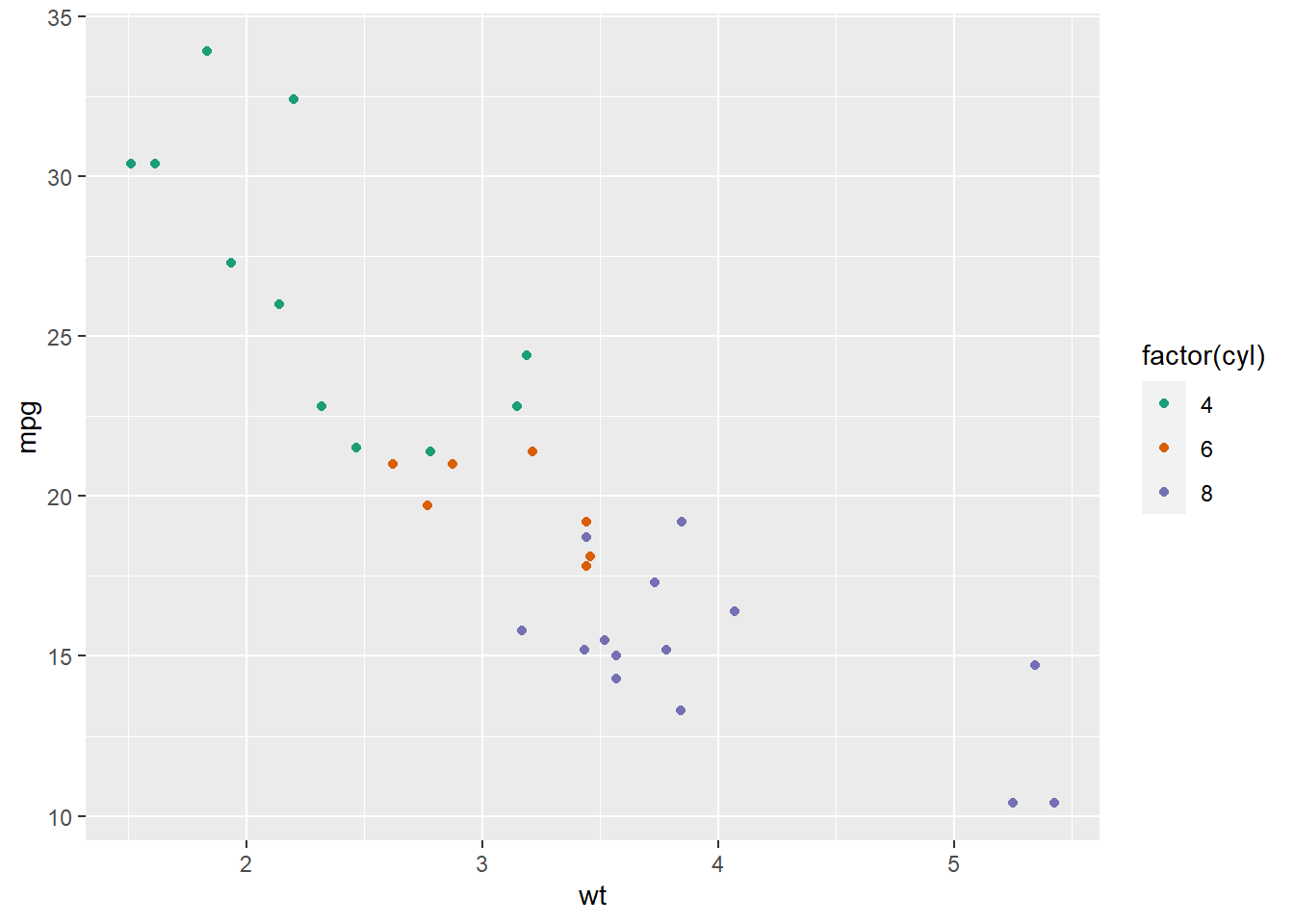

# Viridis color
library(viridis)

## Loading required package: viridisLite

g + scale_color_viridis(discrete = TRUE)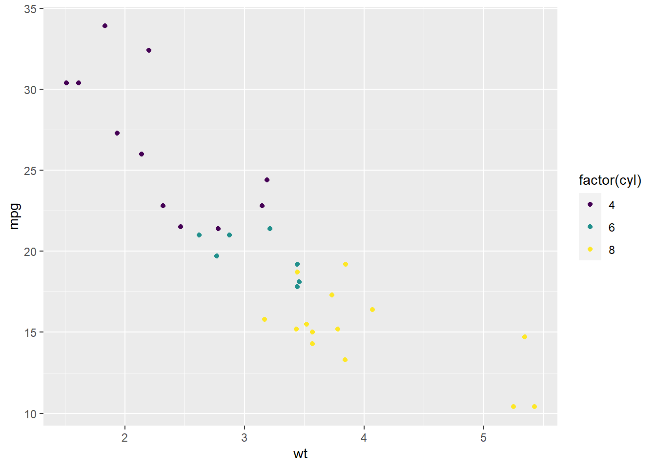

# Grey colors
g + scale_color_grey()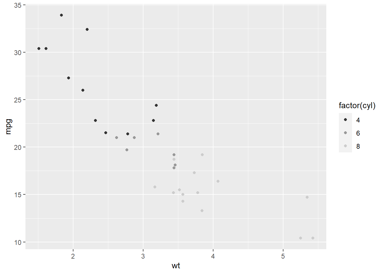

# Manually change colors (`drop` to decide whether to keep unusued factor levels in the scale)
g + scale_color_manual(values = c("#999999", "#E69F00", "#56B4E9"))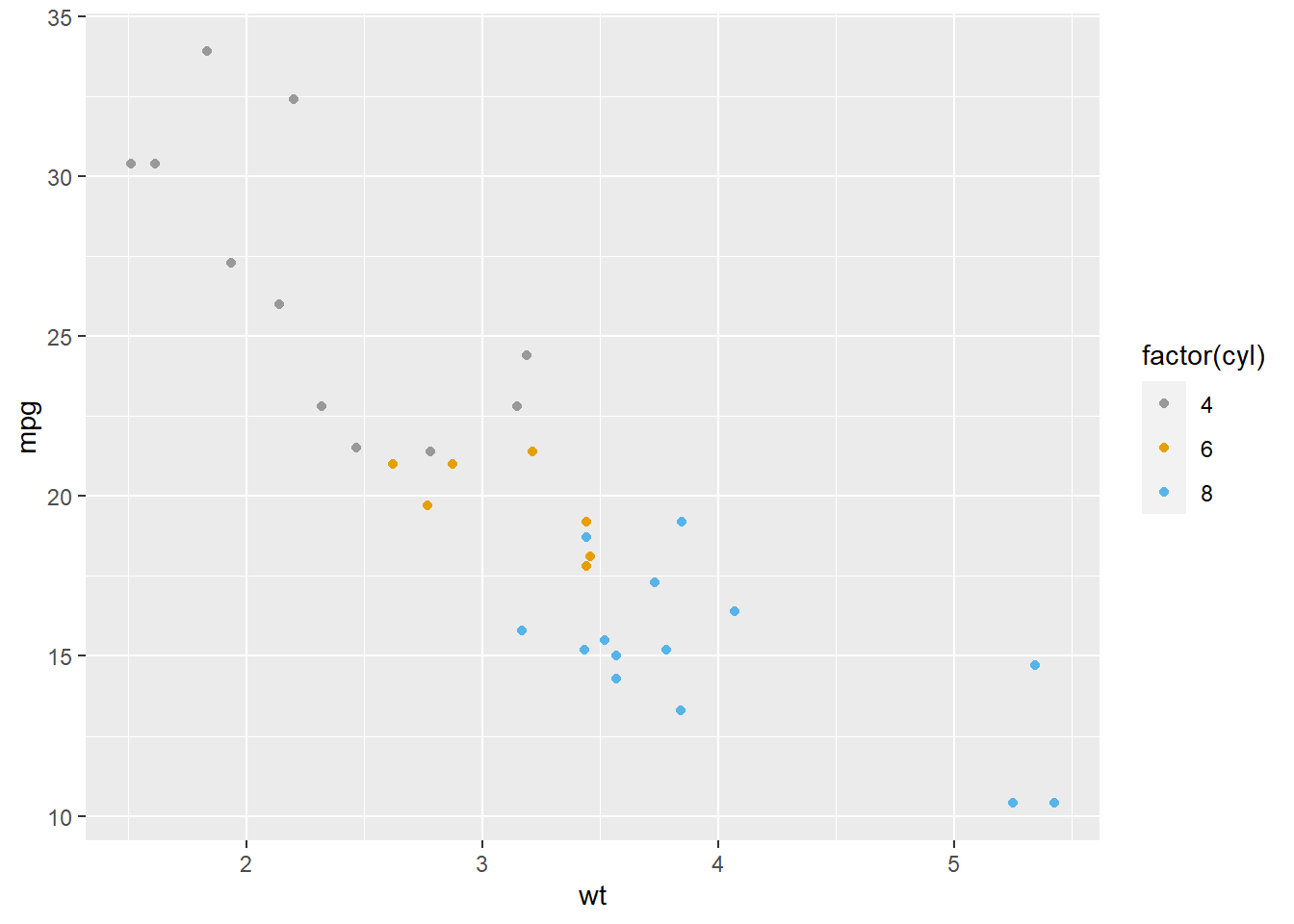

# Argument breaks can be used to control the appearance of the legend
g + scale_color_manual(breaks = c("8", "6", "4"), values = c("red", "blue", "green"))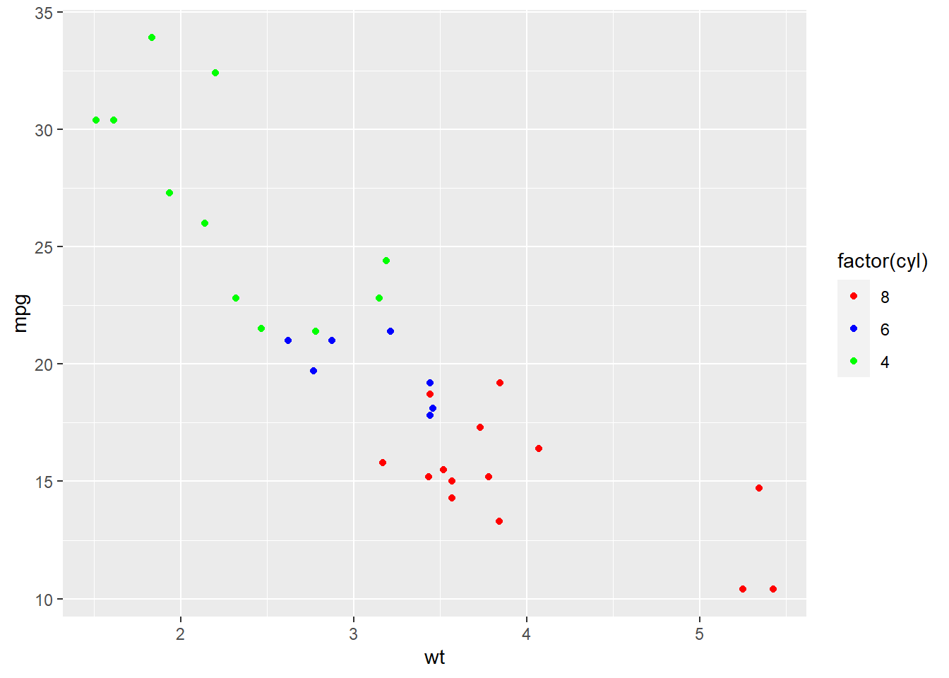

4.2 Continuous colors

# Color by qsec values (default scale_color_gradient())
(g <- ggplot(mtcars, aes(x = wt, y = mpg, color = qsec)) + geom_point())

# RColorBrewer color
# The brewer scales were designed for discrete data but often results to continuous data look good
# The distiller scales extend brewer to continuous scales by smoothly interpolating 7 colours from any palette to a continuous scale
# The fermenter scales provide binned versions of the brewer scales
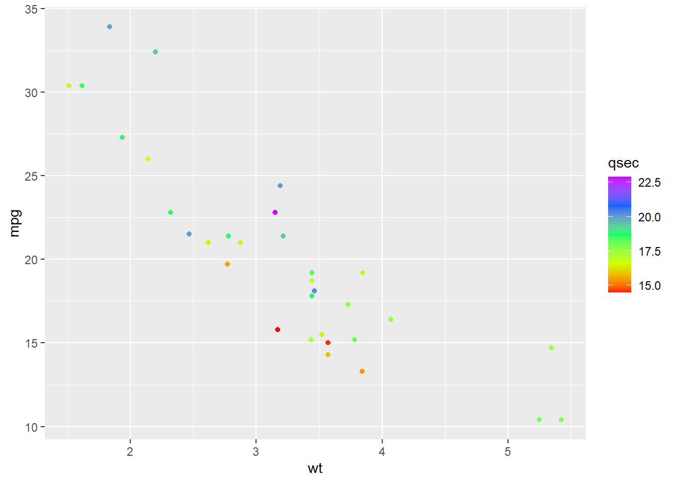
g + scale_color_distiller(palette = "Spectral")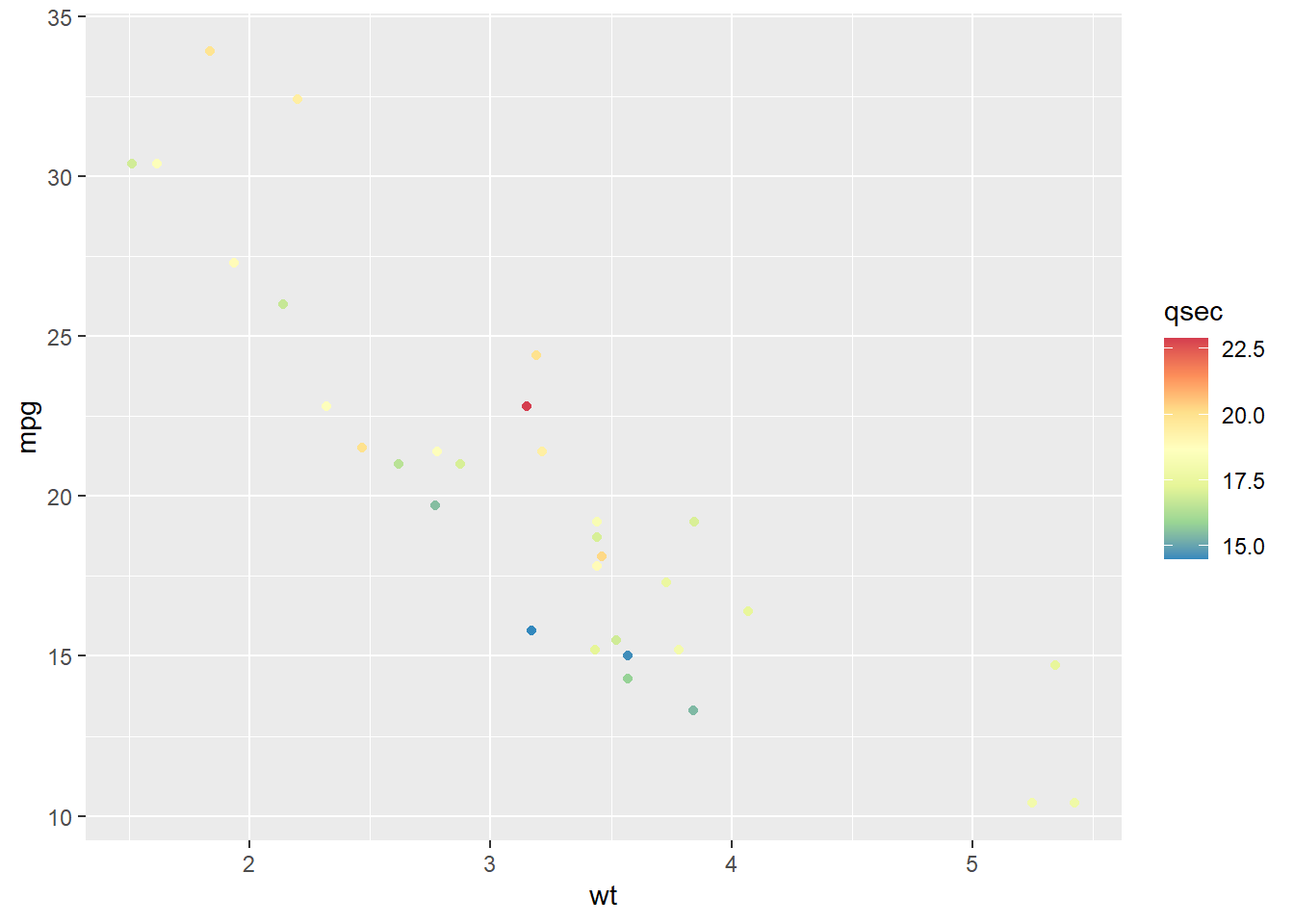

g + scale_color_fermenter(palette = "Spectral")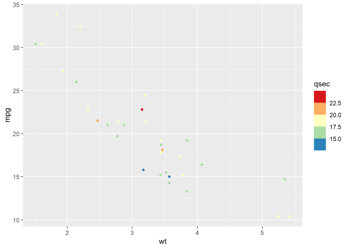

# Viridis color
g + scale_color_viridis()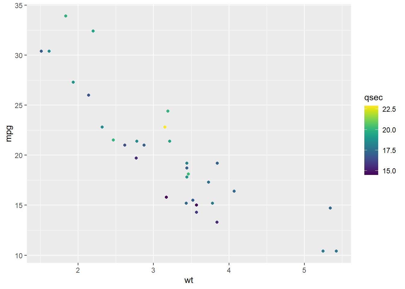

# Sequential gradient low and high colors
g + scale_color_gradient(low = "blue", high = "red")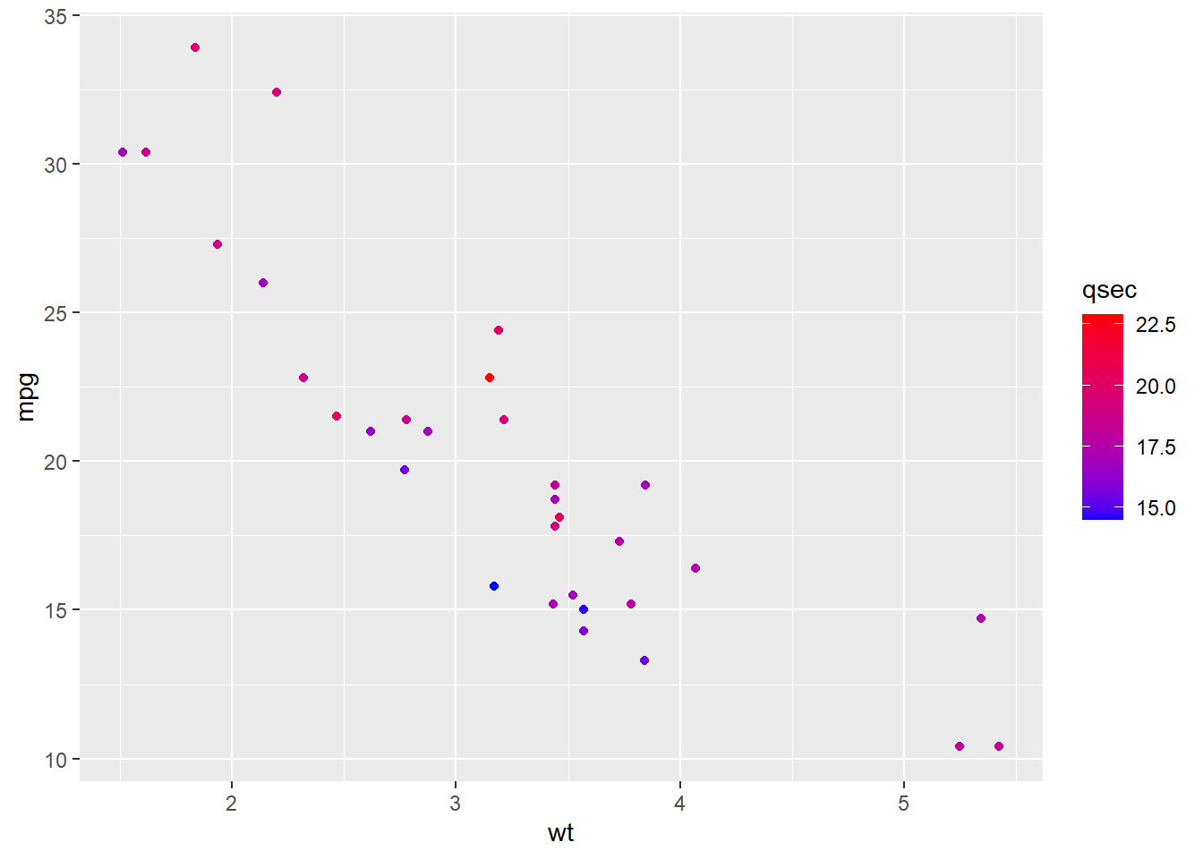

# Diverging gradient between low, mid and high colors
mid <- mean(mtcars$qsec)
g + scale_color_gradient2(midpoint = mid, low = "blue", mid = "white", high = "red")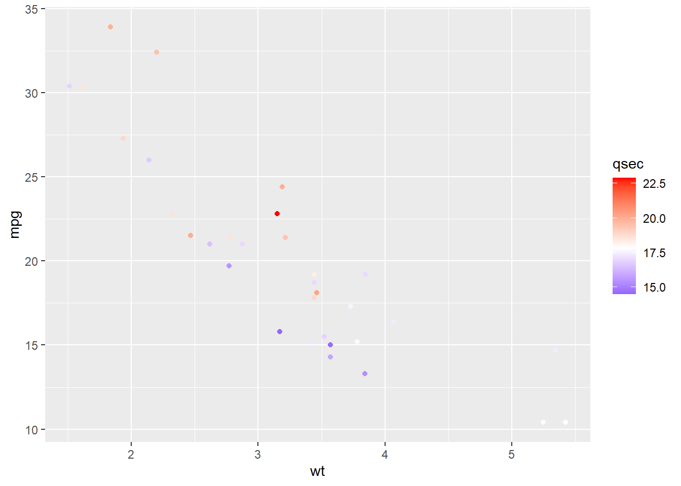

# Gradient between n colors
g + scale_color_gradientn(colours = rainbow(5))