20 Complete spatial randomness

Point processes provide models for point patterns, with complete spatial randomness (CSR) being the simplest theoretical model. CSR assumes that events have an equal likelihood of occurring anywhere within the study area, independent of the locations of other events, which is represented by the homogeneous Poisson process (Diggle 2014). While most processes deviate from CSR to some degree, CSR remains important in investigations, as it helps differentiate between regular and clustered patterns (Figure 20.1). In a random pattern, the distribution of each point is independent of the distribution of the others, and points neither inhibit nor promote one another. Regular patterns have more spacing between points that in a random pattern, possibly due to mechanisms such as competition preventing close occurrences. Clustered patterns exhibit greater aggregation of points than in a random pattern, likely due to processes such as reproduction with limited dispersal or underlying spatial heterogeneity.

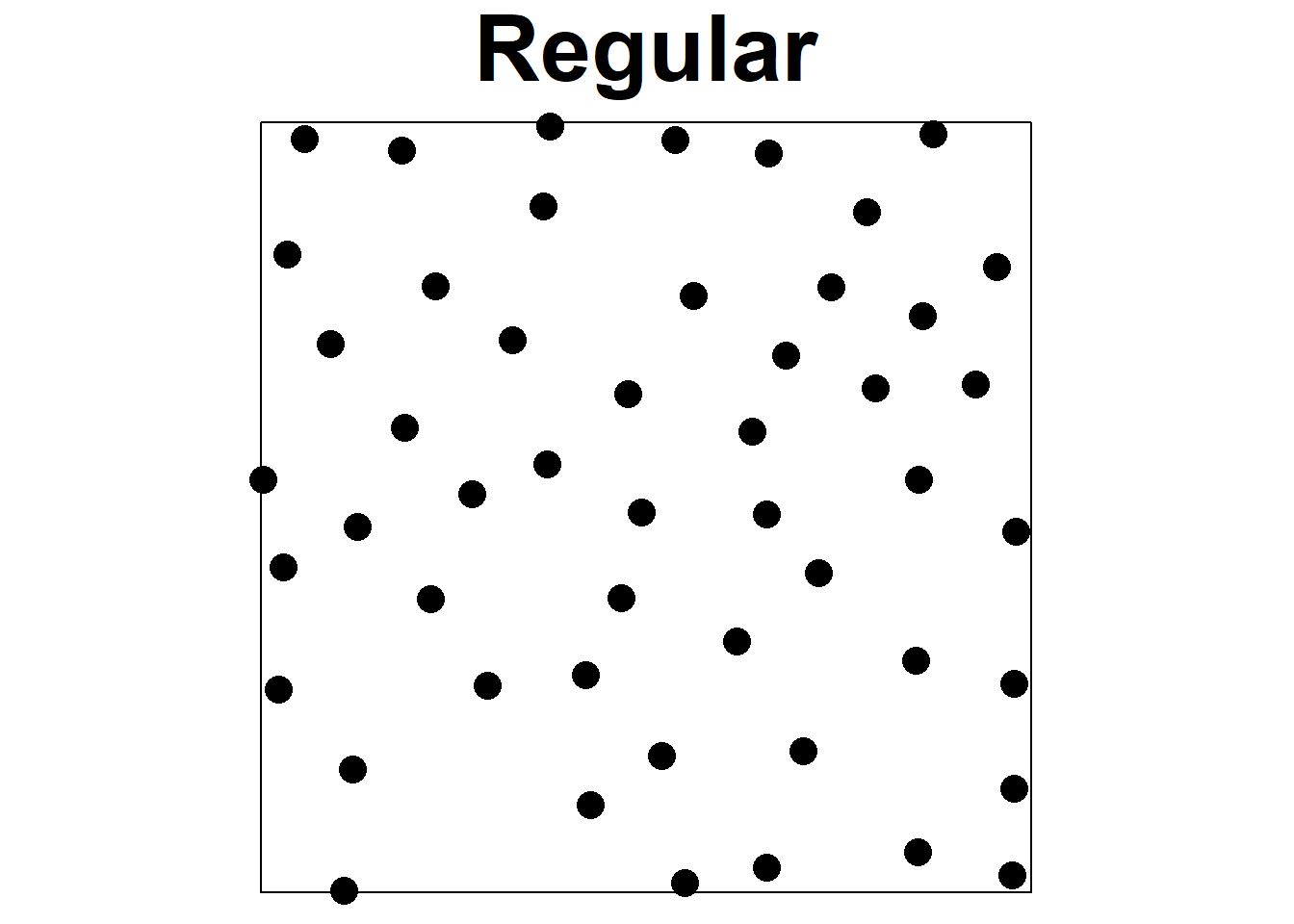
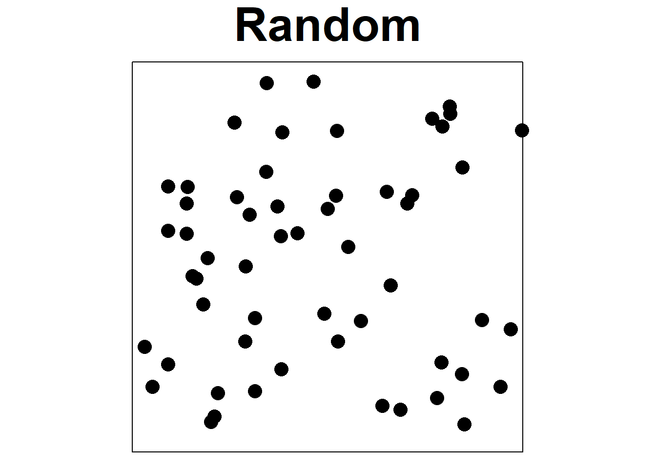
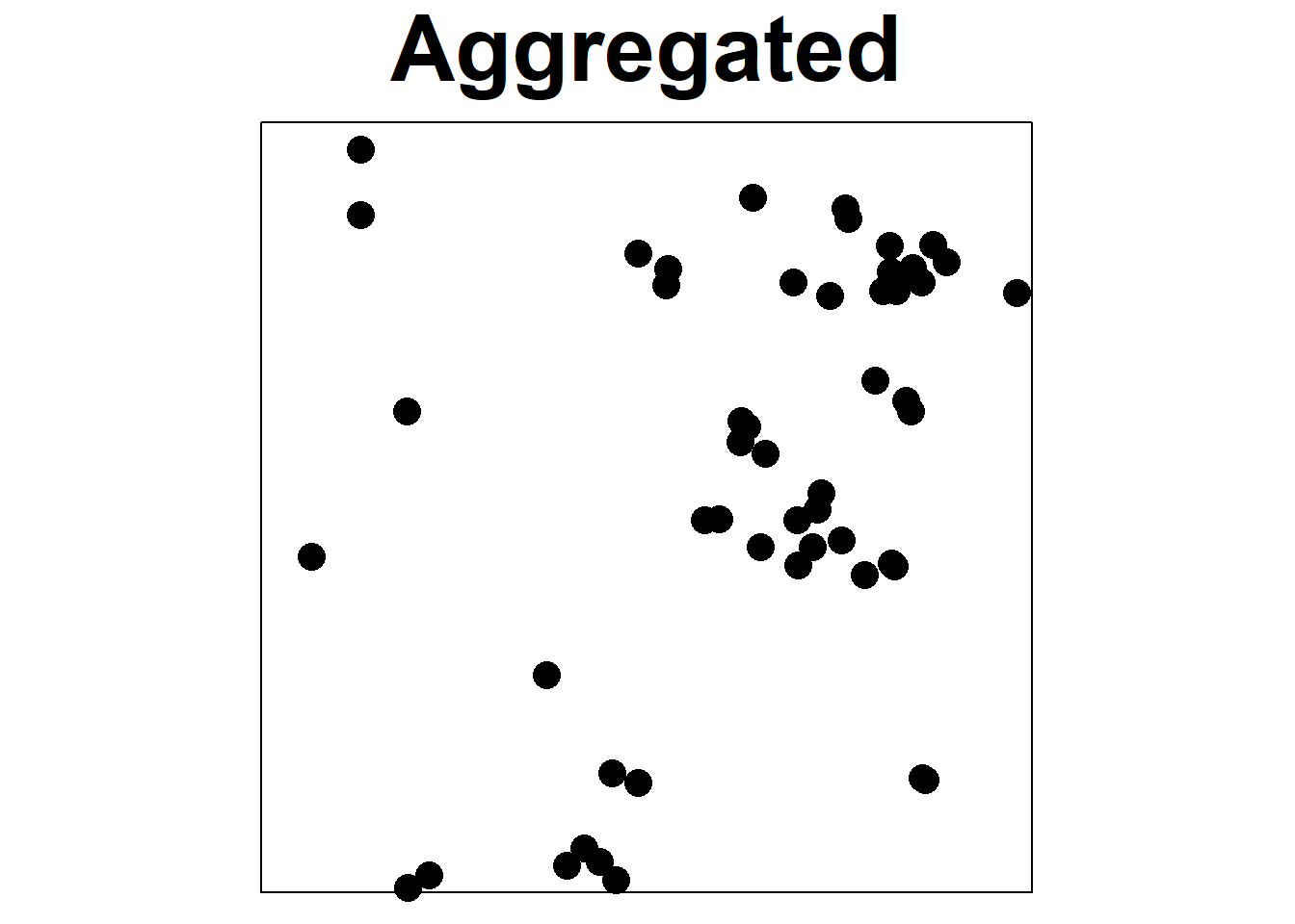
Examples of regular, random, and aggregated point patterns.

FIGURE 20.1: Examples of regular, random, and aggregated point patterns.

20.1 Testing CSR with the quadrat method

Given a point pattern, the first question is often whether there is any evidence to allow rejection of the null hypothesis of complete spatial randomness (CSR). A simple method used to test CSR is the $\chi^2$ test based on quadrat counts.

The quadrat method partitions the study region into $r$ rows and $c$ columns, which define $m = rc$ non-overlapping subregions or quadrats of equal area. This method relies on the fact that, under CSR, the expected number of observations within any region of equal size is the same. Let $n$ be the number of observed points, $m$ the number of quadrats of equal size, and $n_i$ the number of points in quadrat $i$. The expected number of points in each quadrat is $n^* = n/m$. The test statistic is calculated as

\[X^2 = \sum_{i=1}^m \frac{(\mbox{observed}_i - \mbox{expected})^2}{\mbox{expected}} = \sum_{i=1}^m \frac{(n_i - n^*)^2}{n^*}.\]

It can be shown that under CSR, the statistic $X^2$ has a $\chi^2_{m-1}$ distribution. The quadrat method assesses whether CSR is reasonable by comparing the observed value of the $X^2$ statistic to the $\chi^2_{m-1}$ distribution, where $m$ is the number of quadrats. Significance can also be assessed by using Monte Carlo, which involves generating multiple patterns under the null hypothesis, and calculating the $X^2$ statistic for each of them. The p-value is then determined by comparing the $X^2$ statistic for the observed point pattern with the $X^2$ values obtained from the simulations.

Note that the quadrat method’s results may depend on the quadrat’s configuration. In addition, the method tests CSR for the whole point pattern and cannot distinguish different patterns locally. Later, we will see how the K-function can be used to test CSR at a set of distances overcoming these limitations.

20.2 Example

In this example, we show how to use the quadrat.test() function of spatstat (Baddeley, Turner, and Rubak 2022) to test CSR for a given point pattern based on quadrat counts. We use the swedishpines data of spatstat which represents the positions of 71 trees in a Swedish forest plot.

library(spatstat)
data(swedishpines)
X <- swedishpines
X

Planar point pattern: 71 points
window: rectangle = [0, 96] x [0, 100] units (one unit 
= 0.1 metres)

The quadratcount() function of spatstat divides the window containing the point pattern into nx $\times$ ny grid rectangular tiles or quadrats of equal size, and counts the number of points in each quadrat. If the window is not a rectangle, quadrats are intersected with the window. The arguments of the quadratcount() function include X, the point pattern of class ppp, and nx and ny which denote the numbers of rectangular quadrats in the x and y directions (or alternatively xbreaks and ybreaks giving the x and y coordinates, respectively, of the quadrats). Figure 20.2 shows the number of points in each of the quadrats of a 4 $\times$ 3 division of the observation window created with the quadratcount() function.

Q <- quadratcount(X, nx = 4, ny = 3)
Q

             x
y             [0,24) [24,48) [48,72) [72,96]
  [66.7,100]       7       3       6       5
  [33.3,66.7)      5       9       7       7
  [0,33.3)         4       3       6       9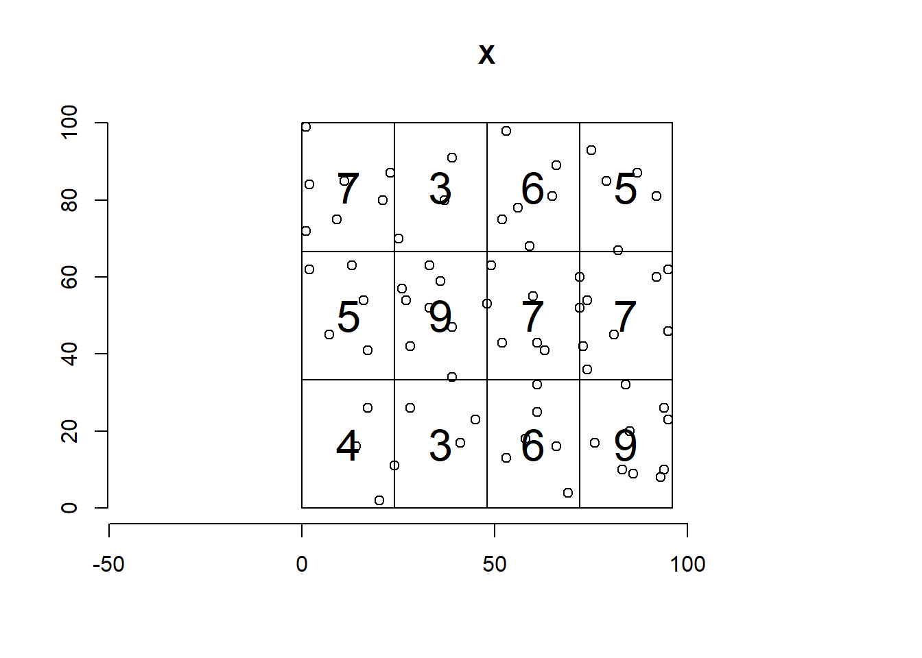

plot(X)
axis(1)
axis(2)
plot(Q, add = TRUE, cex = 2)

$Number of points in each of the quadrats of a 4 $\times$ 3 division of the observation window.$

FIGURE 20.2: Number of points in each of the quadrats of a 4 $\times$ 3 division of the observation window.

The function quadrat.test() performs a test of CSR for a given point pattern. The first argument can be a point pattern of class ppp or the results of applying quadratcount() to a point pattern. The alternative hypothesis is specified in argument alternative and can take the following values:

alternative = "two.sided" tests $H_0$: CSR vs. $H_1$: no CSR (regular or clustered),
alternative = "regular" tests $H_0$: CSR or clustered vs. $H_1$: regular,
alternative = "clustered" tests $H_0$: CSR or regular vs. $H_1$: clustered.

Here, we use quadrat.test() with the default value alternative = "two.sided" to test $H_0$: CSR vs. $H_1$: no CSR (regular or clustered). By default, quadrat.test() assesses significance by comparing the observed test statistic with the chi-squared distribution (method = "Chisq") but can also perform Monte Carlo based tests with method = "MonteCarlo".

quadrat.test(Q)


    Chi-squared test of CSR using quadrat counts

data:  
X2 = 7.6, df = 11, p-value = 0.5
alternative hypothesis: two.sided

Quadrats: 4 by 3 grid of tiles

The observed value of the test statistic is

\[\begin{eqnarray*} X^2 &=& \sum_{i=1}^m \frac{(\mbox{observed}_i - \mbox{expected})^2}{\mbox{expected}} = \sum_{i=1}^m \frac{(n_i - n^*)^2}{n^*} = \\ &=& \frac{(7-n^*)^2+(3-n^*)^2 + \dots + (9-n^*)^2}{n^*} = 7.59 \end{eqnarray*}\]

where $m$ = 12 is the number of regions of equal size, $n_i$ is the number of points in quadrat $i$, $i = 1,\ldots, m$, $n$ = 71 is the number of observed events, and $n^* = n/m = 71/12 = 5.92$ is the expected number of points in each quadrat.

ns <- 71/12
ni <- c(7, 3, 6, 5, 5, 9, 7, 7, 4, 3, 6, 9)
(chi2 <- sum((ni - ns)^2/ns))

[1] 7.592

Under the null hypothesis of CSR, the test statistic has a chi-squared distribution with $m-1 = 12-1$ degrees of freedom. That is, $X^2 \sim \chi^2_{11}$. The p-value is calculated as the probability of obtaining a test statistic as extreme or more extreme than the one observed in the direction of the alternative hypothesis, assuming the null hypothesis is true. If the pattern is regular or clustered, the observed $X^2$ statistic will be near 0 or large. Therefore, the p-value is calculated as 2 times the minimum of the area to the left of the observed $X^2$ and the area to the right of the observed $X^2$:

2*min(pchisq(chi2, 11), 1-pchisq(chi2, 11))

[1] 0.5013

The p-value obtained is greater than the level of significance 0.05. So we fail to reject the null hypothesis and conclude there is no evidence against CSR.

20.3 Alternative hypothesis

Here, we present some examples that use quadrat.test() to test hypotheses with each of the possible values of the argument alternative. Specifically, we use

alternative = "two.sided" to test $H_0$: CSR vs. $H_1$: no CSR (regular or clustered),
alternative = "regular" to test $H_0$: CSR or clustered vs. $H_1$: regular, and
alternative = "clustered" to test $H_0$: CSR or regular vs. $H_1$: clustered.

In each of the examples, the p-value is calculated as the probability of obtaining a test statistic as extreme or more extreme than the one observed in the direction of the alternative hypothesis, assuming the null hypothesis is true. If the calculated p-value is smaller than the significance level $\alpha$, we would reject the null hypothesis. Otherwise, we would fail to reject the null hypothesis.

To test $H_0$: CSR or clustered vs. $H_1$: regular, we use alternative = "regular". If the pattern is regular, the observed $X^2$ statistic will be near 0. Then, the p-value is calculated as the area to the left of the observed $X^2$ (Figure 20.3).

quadrat.test(Q, alternative = "regular")


    Chi-squared test of CSR using quadrat counts

data:  
X2 = 7.6, df = 11, p-value = 0.3
alternative hypothesis: regular

Quadrats: 4 by 3 grid of tiles

# p-value is area to the left of chi2
pchisq(chi2, 11)

[1] 0.2506

To test $H_0$: CSR or regular vs. $H_1$: clustered, we use alternative = "clustered". If the pattern is clustered, the observed $X^2$ statistic will be large, and the p-value is calculated as the area to the right of the observed $X^2$ (Figure 20.3).

quadrat.test(Q, alternative = "clustered")


    Chi-squared test of CSR using quadrat counts

data:  
X2 = 7.6, df = 11, p-value = 0.7
alternative hypothesis: clustered

Quadrats: 4 by 3 grid of tiles

# p-value is area to the right of chi2
1-pchisq(chi2, 11)

[1] 0.7494

Finally, we test $H_0$: CSR vs. $H_1$: no CSR (regular or clustered) using the default value alternative = "two.sided". If the pattern is regular or clustered, the observed $X^2$ statistic will be near 0 or large. The p-value is calculated as 2 times the minimum of the area to the left of the observed $X^2$ and the area to the right of the observed $X^2$.

quadrat.test(Q, alternative = "two.sided") # default


    Chi-squared test of CSR using quadrat counts

data:  
X2 = 7.6, df = 11, p-value = 0.5
alternative hypothesis: two.sided

Quadrats: 4 by 3 grid of tiles

# p-value is 2 times the minimum of
# area to the left of observed chi-squared and
# area to the right of observed chi-squared
2*min(pchisq(chi2, 11), 1-pchisq(chi2, 11))

[1] 0.5013

$Area under the $\chi^2_{11}$ density curve corresponding to the p-value for alternative hypothesis regular (left) and clustered (right).$ $Area under the $\chi^2_{11}$ density curve corresponding to the p-value for alternative hypothesis regular (left) and clustered (right).$

FIGURE 20.3: Area under the $\chi^2_{11}$ density curve corresponding to the p-value for alternative hypothesis regular (left) and clustered (right).

19 Spatial point processes and simulation

21 Intensity estimation