A The R software
A.1 R and RStudio
R is a free and open-source software environment for statistical computing and graphics that provides many excellent packages for importing and manipulating data, statistical analysis, and visualization. R can be downloaded and installed from CRAN (Comprehensive R Archive Network). R can be run using the integrated development environment (IDE) called RStudio which can be freely downloaded from https://posit.co/download/rstudio-desktop/. RStudio includes a console, a syntax-highlighting editor for writing and editing R code, and a variety of tools for data visualization, debugging, and management of files and R projects.
The RStudio IDE has typically four panes (Figure A.1). In the code editor pane (top-left), we create and view the R script files. In the console pane (bottom-left), we see the execution and the output of the R code. To interact with R, we can type commands in the console or write code in script files in the code editor and copy-paste commands to the console. The Environment/History pane (top-right) contains tabs with datasets, variables, and other R objects, as well as the history of the previous R commands executed. This pane may also contain Git options for version control. Finally, the Files/Plots/Packages/Help pane (bottom-right) allows us to see the files in our working directory, the graphs generated, as well as packages and help pages.
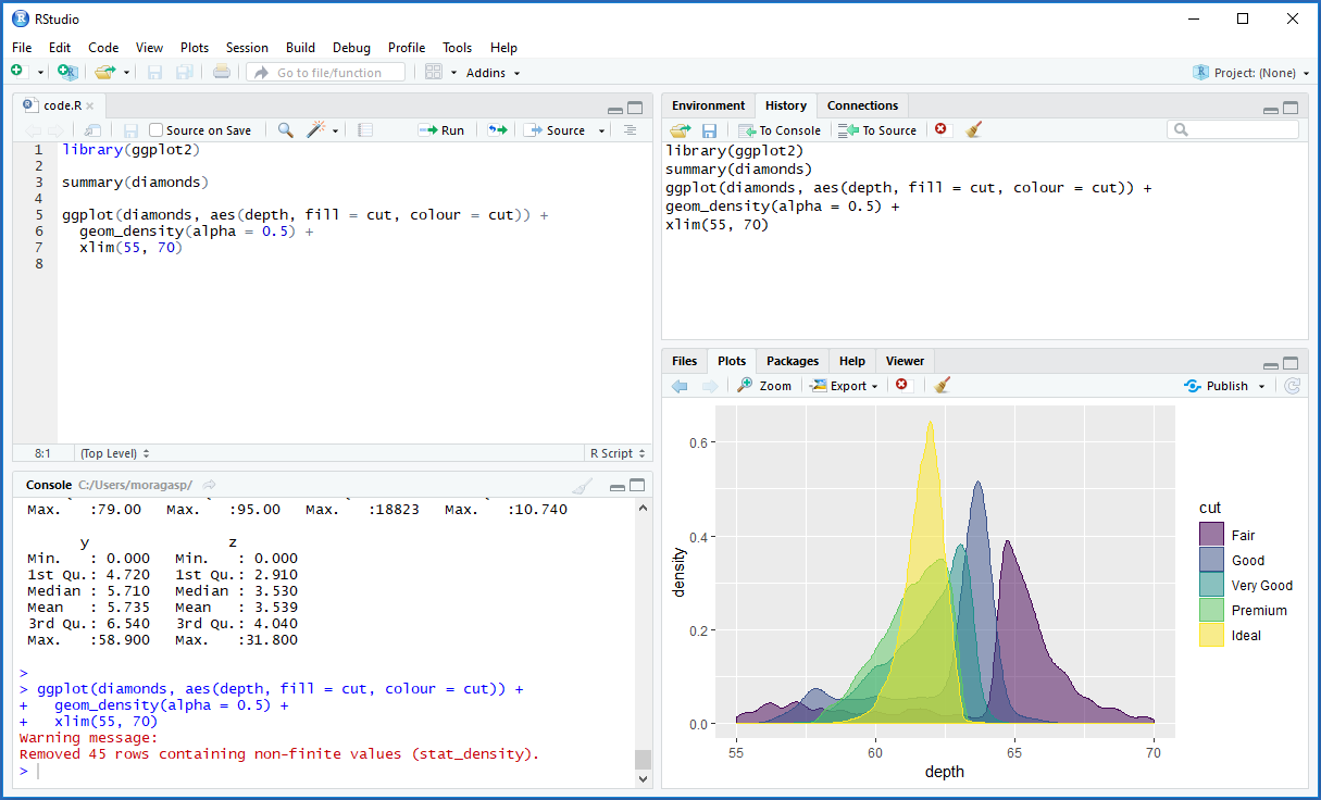
FIGURE A.1: Screenshot of RStudio.
A.2 Installation of R packages
R provides functionality to read and write data; create R objects such as vectors, matrices, data frames and lists; conduct statistical analyses and plotting. We can also install additional R packages for data retrieval, manipulation, analysis, visualization, and reporting. To install an R package from CRAN, we use the install.packages() function passing the name of the package. Then, to use the package, we load it with library(). For example, we can install and load the sf package (Pebesma 2022a) to work with spatial vector data as follows:
install.packages("sf")
library(sf)
A.3 Packages for data visualization
A.3.1 ggplot2
The ggplot2 package (Wickham, Chang, et al. 2022) uses a grammar of graphics which defines the rules of structuring mathematic and aesthetic elements to build graphs layer-by-layer.
To create a plot with ggplot2, we call ggplot() specifying the data frame with the variables to plot (data), and the aesthetic mappings between variables in the data and visual properties of the objects in the graph, such as the position and color of points or lines (mapping = aes()).
Then, we use the + symbol to add layers of graphical components to the graph. Layers consist of geoms, stats, scales, coords, facets, and themes. For example, we add objects to the graph with geom_*() functions (e.g., geom_point() for points, geom_line() for lines). We can also add color scales (e.g., scale_colour_brewer(), faceting specifications (e.g., facet_wrap()), and coordinate systems (e.g., coord_flip()). To save a plot, we use ggsave(). Here, we use the st_read() function of sf to read the shapefile that contains the number of sudden infant deaths in North Carolina, USA, in 1974, and create a map using ggplot2 (Figure A.2).
library(ggplot2)
library(sf)
library(viridis)

d <- st_read(system.file("shape/nc.shp", package = "sf"),
             quiet = TRUE)
ggplot(d) + geom_sf(aes(fill = SID74)) +
  scale_fill_viridis() + theme_bw()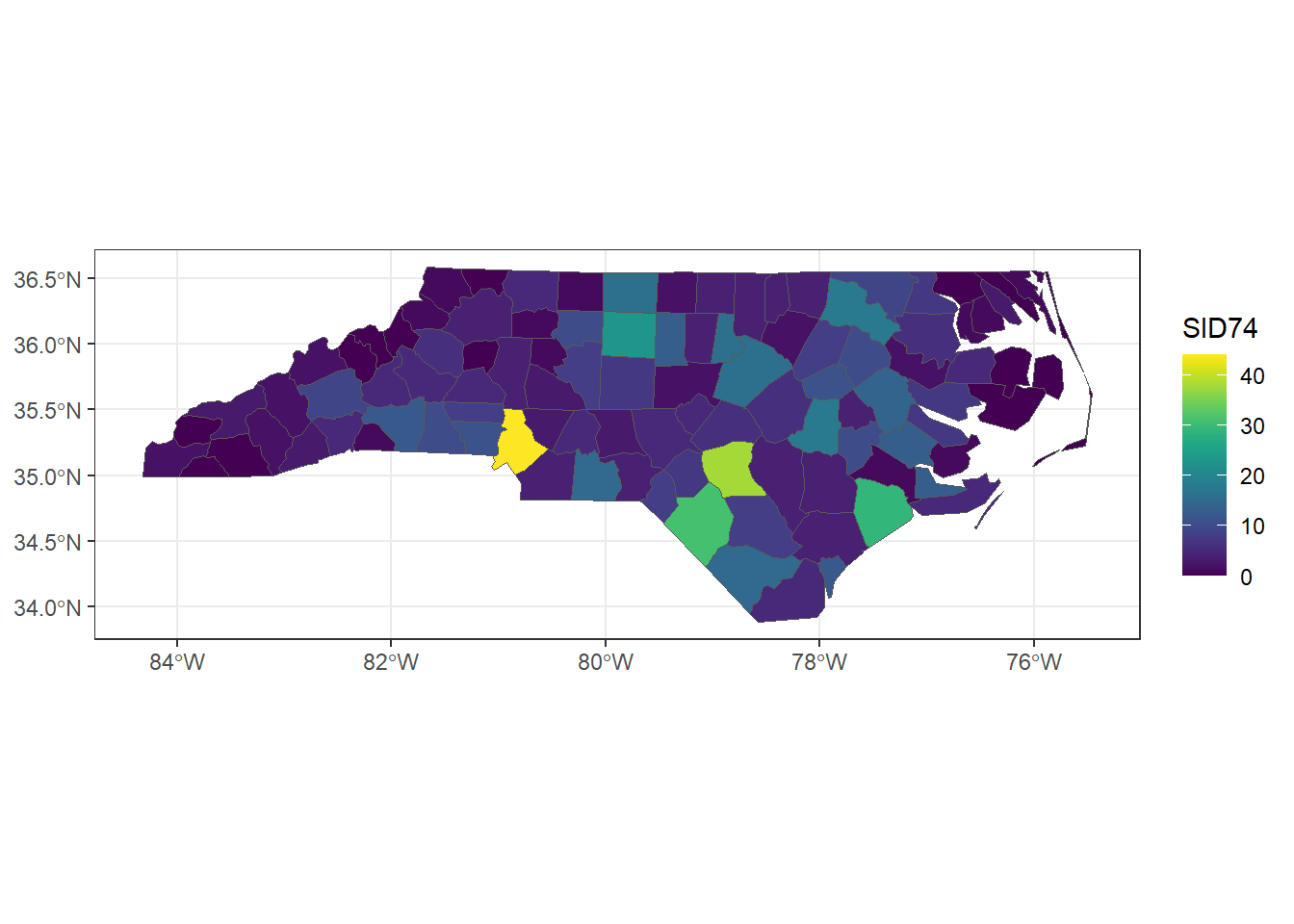
FIGURE A.2: Map of number of sudden infant deaths in North Carolina, USA, in 1974 created with ggplot2.
A.3.2 HTML widgets
HTML widgets are interactive web visualizations built with JavaScript. Here, we provide examples of HTML widgets that allow us to create interactive maps, time series plots and tables. Other examples of HTML widgets can be seen at this website.
The leaflet package (Cheng, Karambelkar, and Xie 2022) allows us to create interactive maps supporting panning and zooming.
We can include basemaps using map tiles to put data into context. A set of available basemaps can be seen here.
Figure A.3 shows a map created with leaflet of the locations and Richter magnitude of seismic events occurred near Fiji in 1964 that are contained in the quakes data.
library(leaflet)
library(sf)

d <- quakes[1:20, ]
pal <- colorNumeric(palette = "YlOrRd", domain = d$mag)
leaflet(d) %>% addTiles() %>%
  addCircleMarkers(color = ~ pal(mag)) %>%
  leaflet::addLegend(pal = pal, values = ~ mag)
FIGURE A.3: Map of the locations and Richter magnitude of seismic events occurred near Fiji in 1964 created with leaflet.
The dygraphs package (Vanderkam et al. 2018) provides functionality to create interactive plots of time series data.
Figure A.4 shows a time series plot created with dygraphs with the mean annual temperature in degrees Fahrenheit in New Haven, Connecticut, USA, over the years contained in the nhtemp data.
library(dygraphs)
dygraph(nhtemp, main = "New Haven Temperatures") %>%
  dyRangeSelector(dateWindow = c("1920-01-01", "1960-01-01"))
FIGURE A.4: Time series plot of the mean annual temperature in degrees Fahrenheit in New Haven, Connecticut, USA, created with dygraphs.
The DT package (Xie, Cheng, and Tan 2022) allows us to display matrices and data frames as tables supporting filtering, pagination and sorting.
For example, the figure below depicts a table created with DT showing the names, and the sepal and petal lengths and widths in centimeters of 150 flowers contained in the iris dataset.
FIGURE A.5: Table created with DT showing the information of the iris dataset.
A.4 Reproducible reports and dashboards
A.4.1 R Markdown
The package rmarkdown (Allaire et al. 2022) allows us to easily turn our analyses into fully reproducible documents that can be shared with others in a variety of formats including HTML and PDF.
An R Markdown document is a text file with extension .Rmd that intermingles text and R code,
and can include narrative text, tables, and visualizations.
When the R Markdown document is compiled, the R code is executed and a report with the output of the R code is created.
Resources to learn R Markdown include Xie, Dervieux, and Riederer (2022), Xie, Allaire, and Grolemund (2018), and chapter 11 of Moraga (2019) which provides a reproducible example of how to create an R Markdown document that includes an exploratory data analysis with tables and visualizations.
A new R Markdown document (.Rmd) can be created by clicking File > New File > R Markdown in RStudio.
From the .Rmd file, a report can be generated using the Knit button in RStudio or executing rmarkdown::render("name.Rmd", "output_document"), where name.Rmd is the name of the .Rmd file, and "output_document" the type of output (e.g., "html_document", "pdf_document").
Note that LaTeX is needed to generate PDF documents. The LaTeX distribution TinyTeX can be installed with the tinytex package (Xie 2022) with
tinytex::install_tinytex() (Xie, Dervieux, and Riederer 2022).
Alternatively, LaTeX can be installed using the resources in the https://www.latex-project.org/get/ website.
An R Markdown document includes three basic components, namely, a YAML header, Markdown text, and R code chunks.
At the beginning of the document, we write
a YAML header surrounded by --- that indicates several options such as title, author, date, and type of output file.
The text is written in Markdown syntax. For example, we can use asterisks for italic text (*text*) and double asterisks for bold text (**text**) .
We can also include equations in LaTeX.
The R code is written within R code chunks which start with three backticks ```{r} and end with three backticks ```.
R code chunks can be specified using several options like
echo=FALSE to hide code and warning=FALSE to supress warnings.
We can include images using knitr::include_graphics("path/img.png") and
tables created with knitr::kable().
We can also include HTML widgets such as objects created with leaflet, DT, and dygraphs.
A.4.2 Quarto
Quarto (Allaire 2022) is a multi-language, next-generation version of R Markdown, that includes many new features and capabilities.
A Quarto document has extension .qmd and can be rendered as formats like PDF and Word using the Render button of RStudio or typing
quarto::quarto_render("name.qmd") in the console.
Quarto is able to render most existing .Rmd files without modification.
Quarto documents are formed of a YAML header, Markdown text, and R code chunks.
The R code chunks options are identified by #| at the beginning of the lines. For example,
A.4.3 Flexdashboard
The flexdashboard package (Sievert, Iannone, et al. 2022) allows us to create dashboards in HTML format that contain several related data visualizations. Examples of dashboards created with flexdashboard can be seen at the RStudio website. Chapter 12 of Moraga (2019) explains how to build a flexdashboard with several components showing air pollution levels in each of the world’s countries (Figure A.6).
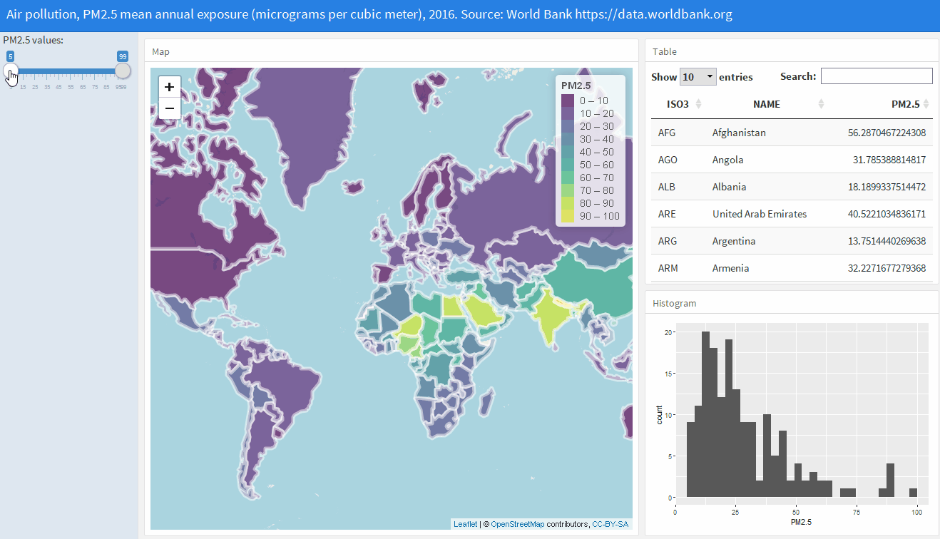
FIGURE A.6: Screenshot of a flexdashboard to visualize air pollution data globally.
To create a flexdashboard, we need to write an R Markdown file with extension .Rmd.
The YAML header of the flexdashboard document needs to have the option output: flexdashboard::flex_dashboard.
Dashboard components are shown according to a layout that specifies the columns and rows.
Columns are included with --------------, and rows for each column with ###.
Layouts can also be specified row-wise rather than column-wise by adding orientation: rows in the YAML.
Layout examples including tabs, multiple pages, and sidebars can be seen at the R Markdown website.
The R code to create the dashboard’s visualizations is written within R code chunks. Dashboards can contain a wide variety of components including images, tables, equations, and HTML widgets. They can also contain value boxes to display single values with titles and icons, and gauges that display values on a meter within a specified range. Moreover, it is also possible to include navigation bars with links to social media, source code, or other links related to the dashboard.
A.4.4 Shiny
Shiny (Chang et al. 2022) is a web application framework for R that enables to build interactive web applications. Examples of Shiny apps can be seen at https://shiny.posit.co/r/gallery/. The SpatialEpiApp package (Moraga 2018b) contains a Shiny app for disease risk estimation, cluster detection, and interactive visualization. Chapters 13-15 of Moraga (2019) provide an introduction to Shiny as well as examples to build a Shiny app to upload and visualize spatial and spatio-temporal data.
A Shiny app can be built by creating a directory that contains an R file with three components. Namely,
a ui user interface object which controls layout and appearance of the app,
a server() function with instructions to build objects displayed in the ui, and a
call to shinyApp() that creates the Shiny app from the ui/server() pair.
# define user interface object
ui <- fluidPage( )
# define server() function
server <- function(input, output){ }
# call to shinyApp() which returns the Shiny app
shinyApp(ui = ui, server = server)
In the ui object, we can include input objects that allow us to interact with the app by modifying their values (e.g., texts, dates, files),
and output objects we want to show in the app (e.g., texts, tables, plots).
The server() function contains the R code to build the outputs. If this code uses an input value, the output will be rebuilt whenever the value changes creating reactivity.
The app directory can also contain data or other R scripts needed by the app.
We can also write two separate files ui.R and server.R for an easier management of code in large apps.
There are two options to share a Shiny app. We can share the R scripts with other users so they can launch the app from R with the runApp() function specifying the path of the directory of the app. Another sharing option that does not require the users to have R is to host the app as a web page at its own URL so the app can be navigated through the internet with a web browser.