13 Spatial interpolation methods

In this chapter, we describe several simple interpolation methods that allow us to predict values of a spatially continuous variable at locations that are not sampled. These methods include closest observation, inverse distance weighting (IDW), and nearest neighbors, and can be easily implemented using the gstat (Pebesma and Graeler 2022) and terra (Hijmans 2022) packages. We also describe an ensemble approach to compute predictions by combining the predictions of several methods.

13.1 Spatial prediction of property prices

13.1.1 Data

To illustrate the spatial interpolation methods, we use the properties data of the spData package (Bivand, Nowosad, and Lovelace 2022) which contains the price of apartments in Athens, Greece, in 2017. properties is a sf object that contains several columns including price with the apartments’ price in Euros, prpsqm with the apartments’ price per square meter, and geometry with the coordinates of the locations. We create a sf object called d with the contents of properties, and a new variable vble with the variable of interest which in this case is price per square meter (prpsqm).

library(spData)
library(sf)
library(terra)
library(tmap)
library(viridis)
d <- properties
d$vble <- d$prpsqm

The object depmunic contains the boundaries of the administrative divisions of Athens. We create a variable map denoting the study region with the union of these boundaries. This is the region where we will predict the variable of interest price per square meter.

map <- st_union(depmunic) %>% st_sf()

The tmap_mode() function of tmap can be used to create static (tmap_mode("plot")) or interactive (tmap_mode("view")) maps. Figure 13.1 shows a static map with the locations and prices of the apartments.

tmap_mode("plot")
tm_shape(map) + tm_polygons(alpha = 0.3) + tm_shape(d) +
  tm_dots("vble", palette = "viridis")

13.1.2 Prediction locations

We wish to predict the prices of properties continuously in space in Athens. To do that, we create a fine raster grid covering Athens and consider the centroids of the raster cells as the prediction locations. We create the raster grid with the rast() function of terra by specifying the region to be covered (map), and the number of rows and columns of the grid (nrows = 100, ncols = 100). The prediction locations are the centroids of the raster cells and can be obtained with the xyFromCell() function of terra. Alternatively, we could create the grid using the st_make_grid() function of sf by specifying the number of grid cells in the horizontal and vertical directions or the cell size.

library(sf)
library(terra)
# raster grid covering map
grid <- terra::rast(map, nrows = 100, ncols = 100)
# coordinates of all cells
xy <- terra::xyFromCell(grid, 1:ncell(grid))

We create a sf object called coop with the prediction locations with st_as_sf() passing the coordinates (as.data.frame(xy)), the name of the coordinates (coords = c("x", "y")), and the coordinate reference system which is the same as the coordinate reference system of map (crs = st_crs(map)). Then, we use st_filter() to keep the locations within the Athens map. Figure 13.1 shows the map with the prediction locations created using the qtm() function of tmap for quick map plots.

coop <- st_as_sf(as.data.frame(xy), coords = c("x", "y"),
                 crs = st_crs(map))
coop <- st_filter(coop, map)

qtm(coop)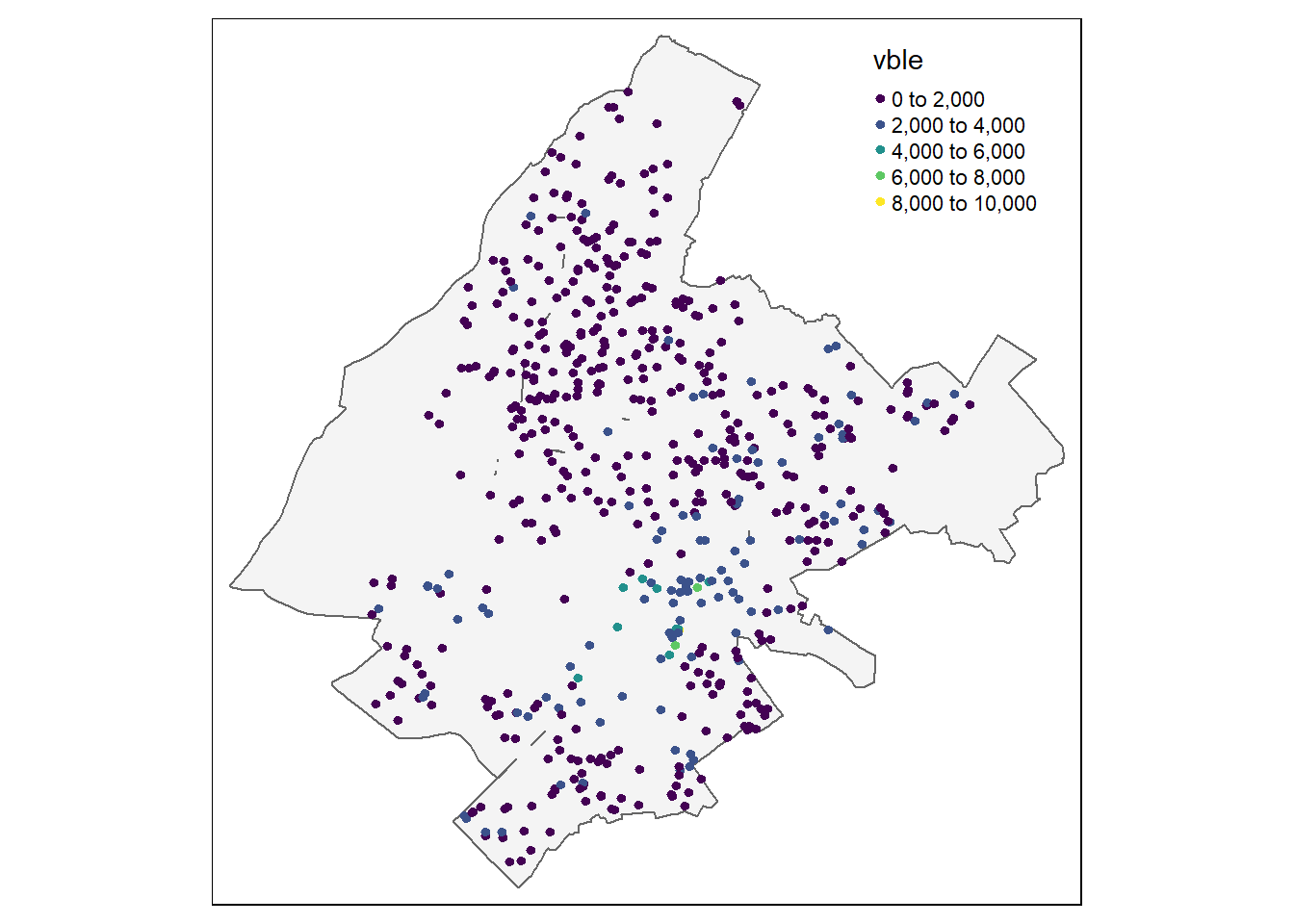

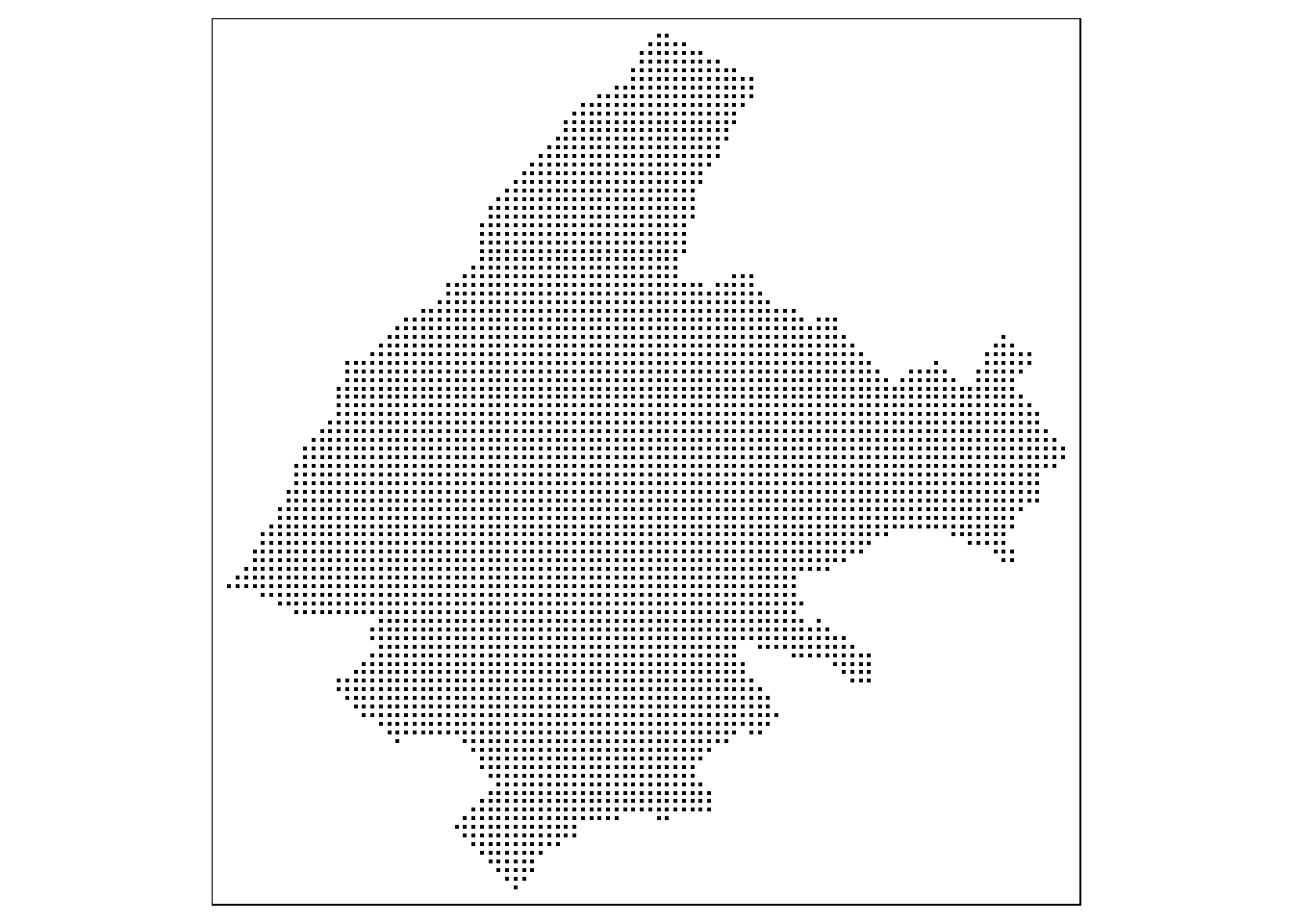
FIGURE 13.1: Top: Locations and prices per square meter of apartments in Athens. Bottom: Prediction locations.

13.1.3 Closest observation

We can obtain predictions at each of the prediction locations as the values of the closest sampled locations. To do that, we can employ the Voronoi diagram (also known as Dirichlet or Thiessen diagram). The Voronoi diagram is created when a region with \(n\) points is partitioned into convex polygons such that each polygon contains exactly one generating point, and every point in a given polygon is closer to its generating point than to any other.

Given a set of points, we can create a Voronoi diagram with the voronoi() function of terra specifying the points as an object of class SpatVector of terra, and map to set the outer boundary of the Voronoi diagram. This returns a Voronoi diagram for the set of points assuming constant values in each of the polygons (Figure 13.2).

Then, we can use the functions tm_shape() and tm_fill() of tmap to plot the values of the variable in each of the polygons indicating the name of the variable col = "vble", the palette palette = "viridis" and the level of transparency alpha = 0.6 (if the plot is interactive).

# Voronoi
v <- terra::voronoi(x = terra::vect(d), bnd = map)
plot(v)
points(vect(d), cex = 0.5)

# Prediction
v <- st_as_sf(v)
tm_shape(v) +
  tm_fill(col = "vble", palette = "viridis", alpha = 0.6)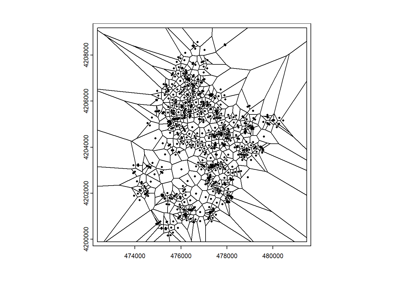

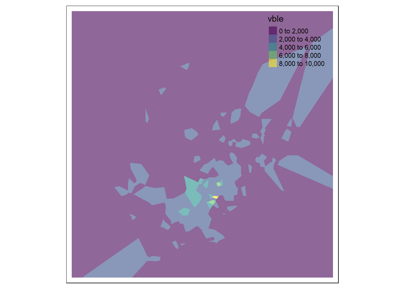
FIGURE 13.2: Left: Voronoi diagram corresponding to the observation locations. Right: Predictions obtained using the closest observation criterion.

We can also extract the predicted values at prediction points coop by using the st_intersection() function of the sf package. Here, instead of creating a map with the predictions at the locations given by coop, we create a map with the predictions at a raster grid. To do that, we transfer the sf object with the predictions at locations coop to the raster grid grid, and create a plot with the raster values with tmap (Figure 13.3).

resp <- st_intersection(v, coop)
resp$pred <- resp$vble

pred <- terra::rasterize(resp, grid, field = "pred", fun = "mean")
tm_shape(pred) + tm_raster(alpha = 0.6, palette = "viridis")

13.1.4 IDW: Inverse Distance Weighting

In the IDW method, values at unsampled locations are estimated as the weighted average of values from the rest of locations with weights inversely proportional to the distance between the unsampled and the sampled locations. Specifically,

\[\hat Z(\boldsymbol{s}_0) = \frac{\sum_{i=1}^n Z(\boldsymbol{s}_i) \times (1/d_i^\beta)}{\sum_{i=1}^n (1/d_i^\beta)} = \sum_{i=1}^n Z(\boldsymbol{s}_i) \times w_i,\]

where \(\hat Z(\boldsymbol{s}_0)\) is the predicted value at \(\boldsymbol{s}_0\), \(n\) the number of sampled locations, \(Z(\boldsymbol{s}_i)\) is the value at location \(\boldsymbol{s}_i\), and \(d_i\) the distance between location \(\boldsymbol{s}_i\) and location \(\boldsymbol{s}_0\) where we want to predict. Here, weights are given by \(w_i = \frac{1/d_i^\beta}{\sum_{i=1}^n (1/d_i^\beta)}\), where \(\beta\) is the distance power that determines the degree to which nearer locations are preferred over more distant locations. For example, if \(\beta = 1\), \(w_i = \frac{1/d_i}{\sum_{i=1}^n (1/d_i)}\).

We can apply the IDW method with the gstat() function of gstat and the following arguments:

• formula: vble ~ 1 to have an intercept only model,
• nmax: number of neighbors is set equal to the total number of locations,
• idp: inverse distance power is set to idp = 1 to have weights with \(\beta = 1\).

Then, we use the predict() function to obtain the predictions and tmap to show the results (Figure 13.3).

library(gstat)
res <- gstat(formula = vble ~ 1, locations = d,
             nmax = nrow(d), # use all the neighbors locations
             set = list(idp = 1)) # beta = 1 

resp <- predict(res, coop)
resp$x <- st_coordinates(resp)[,1]
resp$y <- st_coordinates(resp)[,2]
resp$pred <- resp$var1.pred

pred <- terra::rasterize(resp, grid, field = "pred", fun = "mean")
tm_shape(pred) + tm_raster(alpha = 0.6, palette = "viridis")

13.1.5 Nearest neighbors

In the nearest neighbors interpolation method, values at unsampled locations are estimated as the average of the values of the \(k\) closest sampled locations. Specifically,

\[\hat Z(\boldsymbol{s}_0) = \frac{\sum_{i=1}^k Z(\boldsymbol{s}_i) }{k},\]

where \(\hat Z(\boldsymbol{s}_0)\) is the predicted value at \(\boldsymbol{s}_0\), \(Z(\boldsymbol{s}_i)\) is the observed value corresponding to neighbor \(\boldsymbol{s}_i\), and \(k\) is the number of neighbors considered.

We can compute predictions using nearest neighbors interpolation with the gstat() function of gstat. Here, we consider the number of closest sampled locations equal to 5 by setting nmax = 5. Unlike the IDW method, in the nearest neighbors approach locations further away from the location where we wish to predict are assigned the same weights. Therefore, the inverse distance power idp is set equal to zero so all the neighbors are equally weighted.

Then, we use the predict() function to get predictions at unsampled locations given in coop. Figure 13.3 shows the map with the predictions.

library(gstat)
res <- gstat(formula = vble ~ 1, locations = d, nmax = 5,
             set = list(idp = 0))

resp <- predict(res, coop)
resp$x <- st_coordinates(resp)[,1]
resp$y <- st_coordinates(resp)[,2]
resp$pred <- resp$var1.pred

pred <- terra::rasterize(resp, grid, field = "pred", fun = "mean")
tm_shape(pred) + tm_raster(alpha = 0.6, palette = "viridis")

13.1.6 Ensemble approach

Predictions can also be obtained using an ensemble approach that combines the predictions obtained with several spatial interpolation methods. Specifically, if \(M\) is the number of interpolation methods considered, the predicted value \(\hat Z(\boldsymbol{s}_0)\) can be obtained as

\[\hat Z(\boldsymbol{s}_0) = \sum_{i=1}^M \hat Z^{(i)}(\boldsymbol{s}_0) \times w_i,\]

where \(\hat Z^{(i)}(\boldsymbol{s}_0)\) and \(w_i\) are, respectively, the prediction value and the weight corresponding to method \(i\), with \(i=1,\ldots,M\). The weights can be chosen in different ways. For example, they can be proportional to some goodness-of-fit measure of each method and sum to 1.

Here, we use an ensemble approach to predict the price per square meter of apartments in Athens by combining the predictions of the three previous approaches (closest observation, IDW, nearest neighbors) using equal weights.

The predictions with the closest observation method are obtained using the Voronoi diagram as follows:

# Closest observation (Voronoi)
v <- terra::voronoi(x = terra::vect(d), bnd = map)
v <- st_as_sf(v)
p1 <- st_intersection(v, coop)$vble

The IDW approach can be applied with the gstat() function of gstat specifying nmax as the total number of locations and idp = 1.

# IDW
gs <- gstat(formula = vble ~ 1, locations = d, nmax = nrow(d),
            set = list(idp = 1))
p2 <- predict(gs, coop)$var1.pred

The nearest neighbors method is applied with the gstat() function specifying nmax as the number of neighbors and with equal weights (idp = 0).

# Nearest neighbors
nn <- gstat(formula = vble ~ 1, locations = d, nmax = 5,
            set = list(idp = 0))
p3 <- predict(nn, coop)$var1.pred

Finally, the ensemble predictions are obtained by combining the predictions of these three methods with equal weights.

# Ensemble (equal weights)
weights <- c(1/3, 1/3, 1/3)
p4 <- p1 * weights[1] + p2 * weights[2] + p3 * weights[3]

We create a map with the predictions by creating a raster with the predictions and using the tmap package (Figure 13.3).

resp <- data.frame(
x = st_coordinates(coop)[, 1],
y = st_coordinates(coop)[, 2],
pred = p4)

resp <- st_as_sf(resp, coords = c("x", "y"), crs = st_crs(map))

pred <- terra::rasterize(resp, grid, field = "pred", fun = "mean")
tm_shape(pred) + tm_raster(alpha = 0.6, palette = "viridis")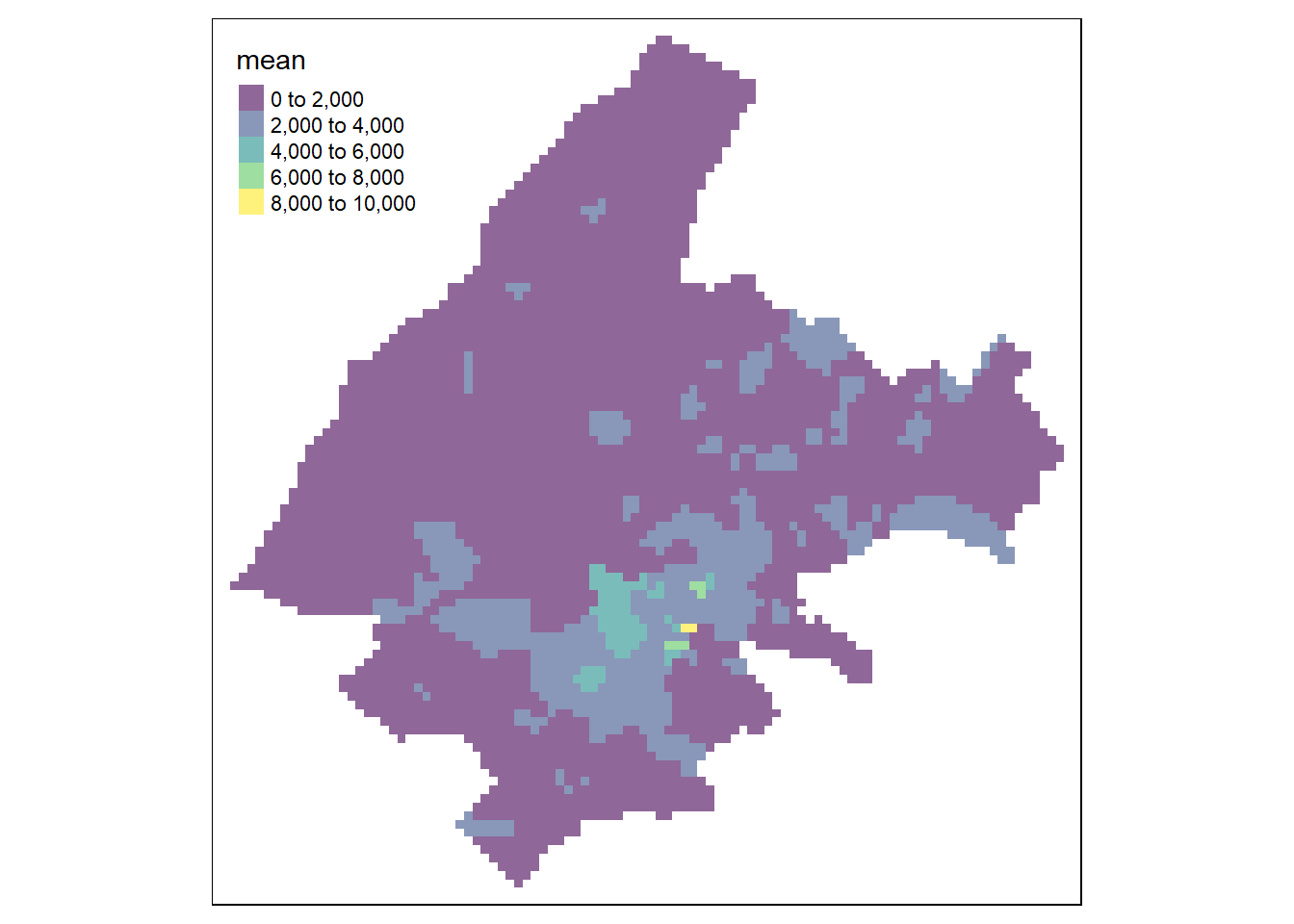

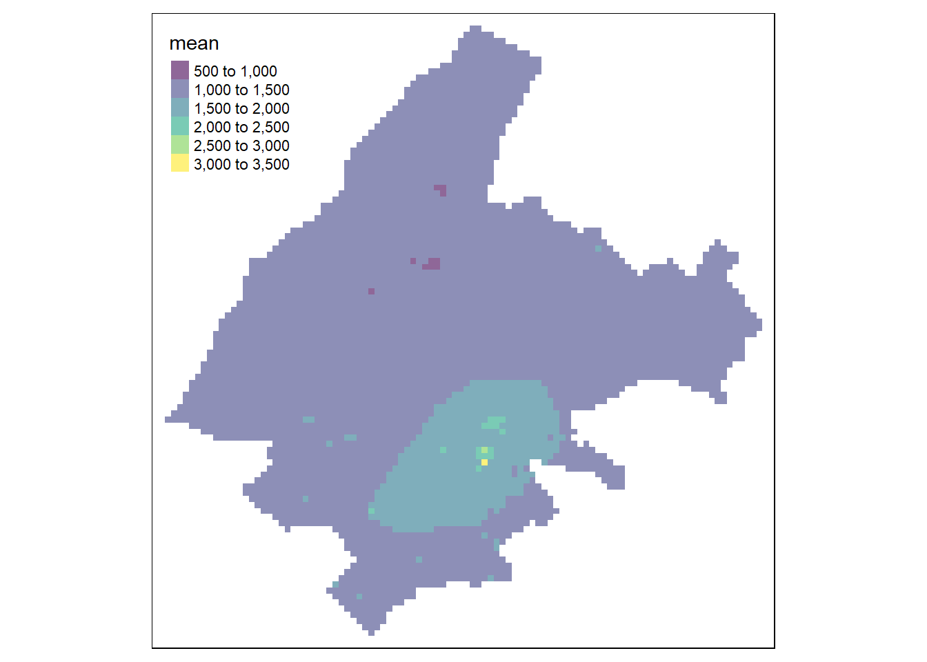
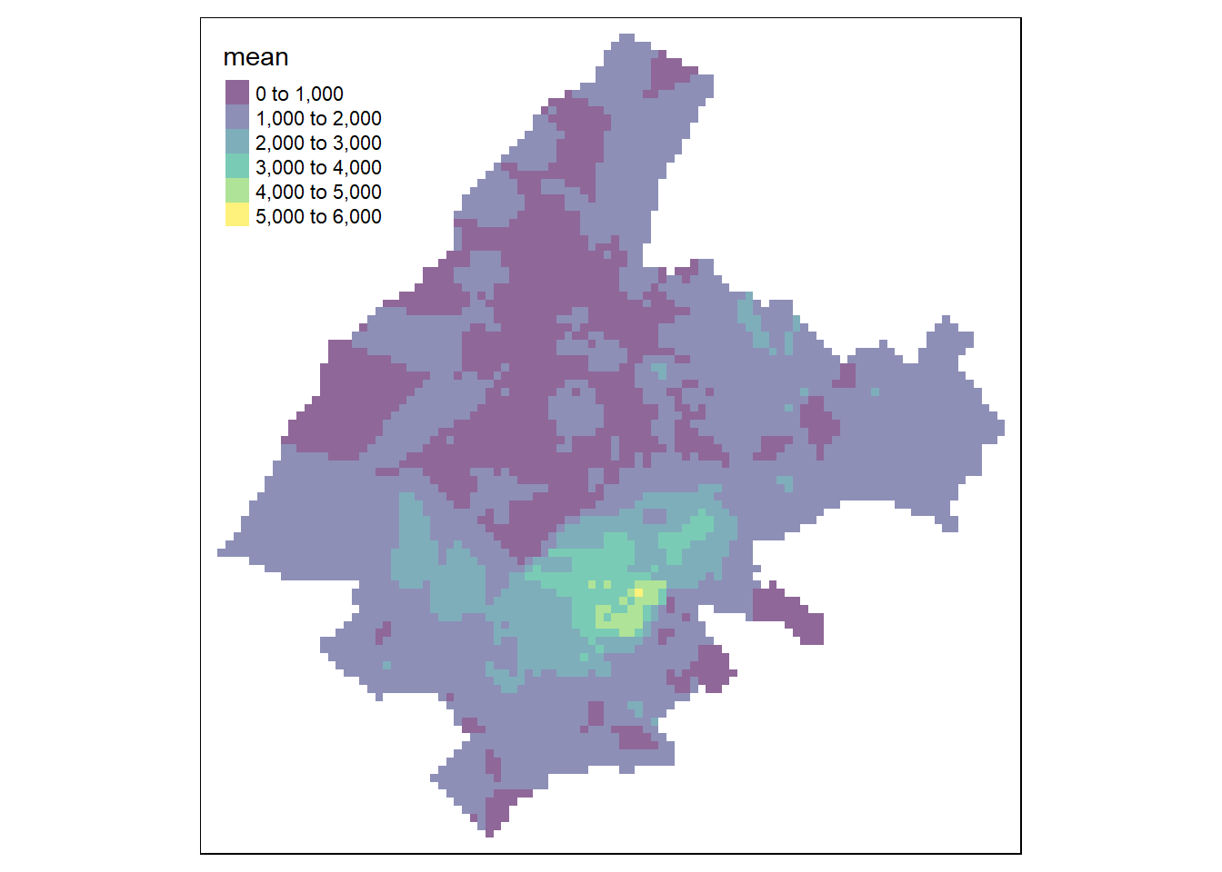
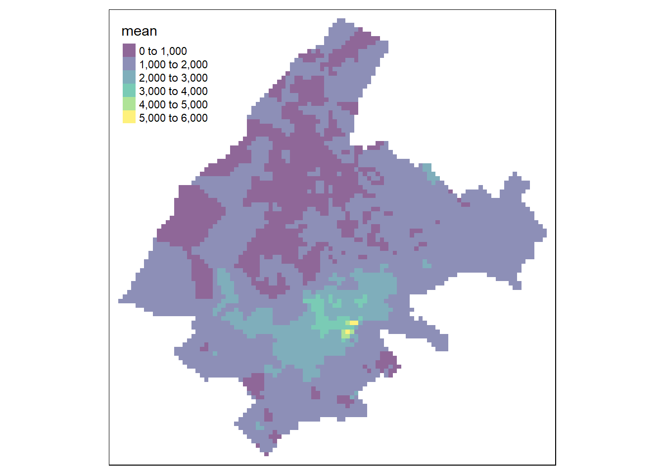
FIGURE 13.3: Predictions obtained using closest observation (top-left), IDW (top-right), nearest neighbors (bottom-left), and ensemble approach (bottom-right).

13.1.7 Cross-validation

We can assess the performance of each of the methods presented above using \(K\)-fold cross-validation and the root mean squared error (RMSE). First, we split the data in \(K\) parts. For each part, we use the remaining \(K-1\) parts (training data) to fit the model and that part (testing data) to predict. We compute the RMSE by comparing the testing and predicted data in each of the \(K\) parts:

\[RMSE = \left(\frac{1}{n_{test}} \sum_{i=1}^{n_{test}} (y_i^{test} - \widehat{y_i^{test}})^2 \right)^{1/2},\]

where \(y_i^{test}\) and \(\widehat{y_i^{test}}\) are the observed and predicted values of observation \(i\) in the test set, and \(n_{test}\) is the number of observations in the test set. Finally, we average the \(RMSE\) values obtained in each of the \(K\) parts.

Note that if \(K\) is equal to the number of observations \(n\), this procedure is called leave-one-out cross-validation (LOOCV). That means that \(n\) separate data sets are trained on all of the data except one observation, and then prediction is made for that one observation.

Here, we assess the performance of each of the methods previously employed to predict the prices of apartments in Athens. We create training and testing sets by using the dismo:kfold() function of the dismo package (Hijmans et al. 2022) to randomly assign the observations to \(K = 5\) groups of roughly equal size. For each group, we fit the model using the training data, and obtain predictions of the testing data. We calculate the RMSEs of each part and average the RMSEs to obtain a \(K\)-fold cross-validation estimate.

set.seed(123)

# Function to calculate the RMSE
RMSE <- function(observed, predicted) {
sqrt(mean((observed - predicted)^2))
}

# Split data in 5 sets
kf <- dismo::kfold(nrow(d), k = 5) # K-fold partitioning

# Vectors to store the RMSE values obtained with each method
rmse1 <- rep(NA, 5) # Closest observation
rmse2 <- rep(NA, 5) # IDW
rmse3 <- rep(NA, 5) # Nearest neighbors
rmse4 <- rep(NA, 5) # Ensemble

for(k in 1:5) {
# Split data in test and train
test <- d[kf == k, ]
train <- d[kf != k, ]

# Closest observation
v <- terra::voronoi(x = terra::vect(train), bnd = map)
v <- st_as_sf(v)
p1 <- st_intersection(v, test)$vble
rmse1[k] <- RMSE(test$vble, p1)

# IDW
gs <- gstat(formula = vble ~ 1, locations = train,
            nmax = nrow(train), set = list(idp = 1))
p2 <- predict(gs, test)$var1.pred
rmse2[k] <- RMSE(test$vble, p2)

# Nearest neighbors
nn <- gstat(formula = vble ~ 1, locations = train,
            nmax = 5, set = list(idp = 0))
p3 <- predict(nn, test)$var1.pred
rmse3[k] <- RMSE(test$vble, p3)

# Ensemble (weights are inverse RMSE so lower RMSE higher weight)
w <- 1/c(rmse1[k], rmse2[k], rmse3[k])
weights <- w/sum(w)
p4 <- p1 * weights[1] + p2 * weights[2] + p3 * weights[3]
rmse4[k] <- RMSE(test$vble, p4)
}

The RMSE values obtained in each of the 5 splits are shown below. We see the minimum average RMSE corresponds to the ensemble method.

# RMSE obtained for each of the 5 splits
data.frame(closest.obs = rmse1, IDW = rmse2,
           nearest.neigh = rmse3, ensemble = rmse4)

  closest.obs   IDW nearest.neigh ensemble
1       960.0 855.1         819.8    732.7
2       836.8 762.7         700.7    678.1
3      1038.5 962.8         867.1    868.9
4      1003.1 921.6         870.3    843.2
5       803.5 844.2         783.0    717.8

# Average RMSE over the 5 splits
data.frame(closest.obs = mean(rmse1), IDW = mean(rmse2),
           nearest.neigh = mean(rmse3), ensemble = mean(rmse4))

  closest.obs   IDW nearest.neigh ensemble
1       928.4 869.3         808.2    768.2