16 Methods assessment

The predictive performance of a spatial interpolation method can be assessed in several ways. For example, we can compare the observations and the predictions made at a set of locations using the Mean Absolute Error (MAE), the Root Mean Squared Error (RMSE), and the 95% Coverage Probability (CP).

Let \(y_i\) and \(\hat y_i\) be the observed and predicted values, respectively, at locations \(x_i\), \(i=1,\ldots, m\). We can calculate the Mean Absolute Error as

\[MAE = \frac{1}{m}\sum_{i=1}^m |y_i - \hat y_i|,\] and the Root Mean Squared Error as

\[RMSE = \left( \frac{1}{m} \sum_{i=1}^m (y_i - \hat y_i)^2 \right)^{1/2}.\] The 95% coverage probability is the proportion of times that the observed values are within their corresponding 95% prediction intervals and can be calculated as

\[\frac{1}{m} \sum_{i=1}^m I\left(y_i \in PI^{95\%}_i \right),\] where \(I\left(y_i \in PI^{95\%}_i \right)\) is an indicator function that takes the value 1 if \(y_i\) is inside its 95% prediction interval \(PI^{95\%}_i\), and 0 otherwise.

If the spatial interpolation method provides prediction distributions, the Continuous Ranked Probability Score (CRPS) can be used to compare observations and predictions accounting for the uncertainty (Matheson and Winkler 1976). The CRPS for observation \(y\) is a score function that compares the Cumulative Distribution Function (CDF) of the prediction distribution (\(F\)) with the degenerate CDF of the observation (\(1{\{u \geq y\}}\)):

\[CRPS(F, y) = \int_{-\infty}^{+\infty} \left(F(u) - 1{\{u\geq y\}} \right)^2 du.\]

Figure 16.1 shows a plot representing the CRPS for a given observation. Note that a good method would yield a predicted distribution close to the observed value. Therefore, the preferred method would be one where the squared area between the two CDFs is small.

The CRPS for a set of observations can be calculated by aggregating the CRPS of the individual observations using an average or weighted average. A perfect CRPS score is equal to 0. Note that the CRPS reduces to the MAE if the predicted distribution is just a point estimate and not a distribution.

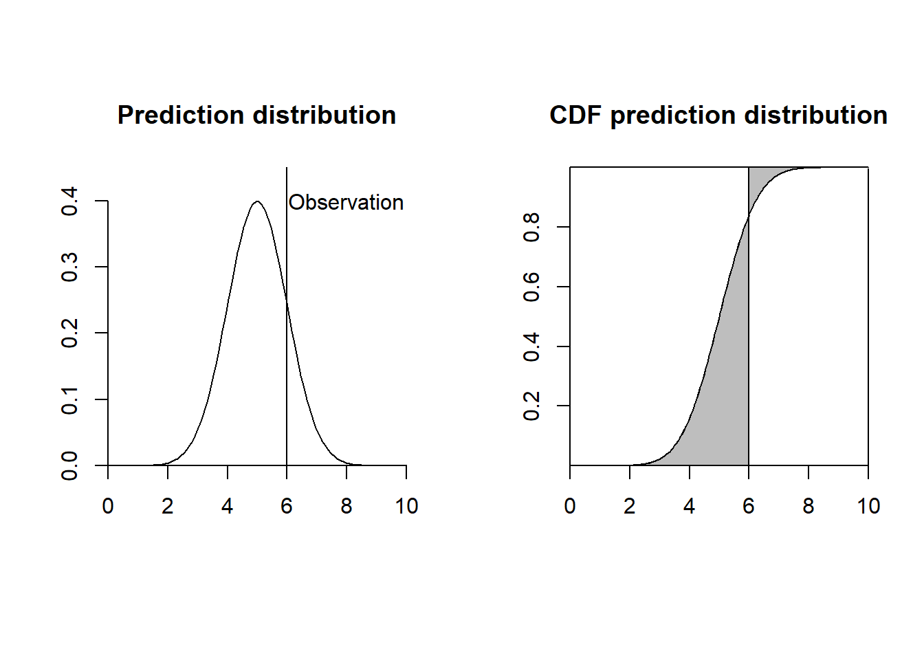
FIGURE 16.1: Left: Observation and prediction distribution. Right: Continuous Ranked Probability Score (CRPS) represented as the gray area between the cumulative distribution functions.

16.1 Cross-validation

The performance indices presented above can be computed using a new dataset or by splitting an existing dataset into a training dataset to fit the model and a testing dataset for validation. In cross-validation, the data is randomly split into several disjoint folds. Then, each fold is put aside in turn and used to evaluate the predictions obtained from a model fitted on the remaining folds. This procedure is called \(K\)-fold cross-validation if the data is split into \(K\) folds, and leave-one-out cross-validation (LOOCV) if each fold consists of only one observation.

In applications where spatial autocorrelation is present, randomly splitting the data into training and testing datasets may lead to an overestimation of the predictive performance since the characteristics of the testing and training datasets could be similar. In these situations, better performance measures may be used by employing spatial cross-validation and probability sampling.

Spatial cross-validation generates training and testing locations that are enough separated to provide independent datasets. For example, the blockCV package (Valavi et al. 2023) provides a range of functions to generate spatially and environmentally separated datasets for spatial K-fold and LOOCV. The package includes functions to construct spatial and buffer blocks, and to allocate them to cross-validation folds. It also has functionality to assess the level of spatial autocorrelation to help select the blocks and the buffer sizes appropriately.

Note also that spatial cross-validation techniques may generate training datasets where geographic and therefore covariate space is excluded causing under-representation of environmental conditions similar to those at the validation locations. Probability sampling can be used in these situations to obtain a more representative set of locations and avoid extrapolation problems (Wadoux et al. 2021).