21 Intensity estimation

The intensity function of a spatial point process \(\{X_1, X_2, \ldots, X_{N(A)}\}\) in a planar window \(A \subset \mathbb{R^2}\) is defined as

\[\lambda(\boldsymbol{x}) = \lim_{|d\boldsymbol{x}| \rightarrow 0} \frac{E[N(d\boldsymbol{x})]}{|d\boldsymbol{x}|},\] where \(d\boldsymbol{x}\) is a small region containing the point \(\boldsymbol{x}\). Given a stationary and isotropic spatial point process, the intensity function is constant equal to the expected number of events per unit area:

\[\lambda(\boldsymbol{x}) = \lambda = \frac{E[N(A)]}{|A|}.\]

Thus, for an observed spatial point pattern of \(n\) events observed in a region \(A\), the intensity can be estimated as the observed number of events per unit area:

\[\hat \lambda = \frac{n}{|A|}\]

For non-stationary processes, a common method to estimate the spatially varying intensity function involves kernel density estimation (Silverman 1986; González and Moraga 2023b). Usually, kernel estimation methods focus on estimating the probability density function \(f(\cdot)\) rather than the intensity function \(\lambda(\cdot)\). The density function defines the probability of observing an event at a location \(\boldsymbol{x}\) and integrates to one across the area of study. In contrast, the intensity function provides the number of events expected per unit area at location \(\boldsymbol{x}\) and integrates to the overall mean number of events per unit area. As a result, the density and intensity functions are proportional:

\[\lambda(\boldsymbol{x}) = f(\boldsymbol{x}) \int_A \lambda(\boldsymbol{u})d\boldsymbol{u},\]

where \(\int_A \lambda(\boldsymbol{u})d\boldsymbol{u}\) is the expected number of events in \(A\). Then, the relative spatial pattern in densities and intensities are the same.

Kernel estimators of the density function \(f(\cdot)\) and the intensity function \(\lambda(\cdot)\) at the location \(\boldsymbol{x}\) based on the observed events \(\{\boldsymbol{x}_1, \ldots, \boldsymbol{x}_n\}\) take the form

\[\begin{eqnarray*} \hat f(\boldsymbol{x}) &=& \frac{1}{n} \sum_{i=1}^n \frac{1}{h^2} K\left(\frac{\boldsymbol{x}-\boldsymbol{x}_i}{h}\right) \mbox{ and } \\ \hat \lambda(\boldsymbol{x}) &=& \sum_{i=1}^n \frac{1}{h^2} K\left(\frac{\boldsymbol{x}-\boldsymbol{x}_i}{h}\right), \end{eqnarray*}\]

where \(K(\cdot)\) is a symmetric function such that \(K(\boldsymbol{x}) \geq 0\) \(\forall \boldsymbol{x}\) and \(\int_A K(\boldsymbol{x}) d\boldsymbol{x} = 1\) known as kernel, and \(h\) is a smoothing parameter known as “bandwidth” (Figure 21.1).

Edge effects tend to distort the kernel estimates close to the boundary of the region, since events near the boundary have fewer local neighbors than events in the interior. One way to deal with this problem is to modify the kernel estimate by dividing by the following edge-correction term:

\[p_h(\boldsymbol{x}) = \int_A h^{-2} K\left(\frac{\boldsymbol{x}-\boldsymbol{u}}{h}\right)d\boldsymbol{u},\]

which represents the volume under the scaled kernel centered on \(\boldsymbol{x}\) which lies inside the study region (Gatrell et al. 1996).

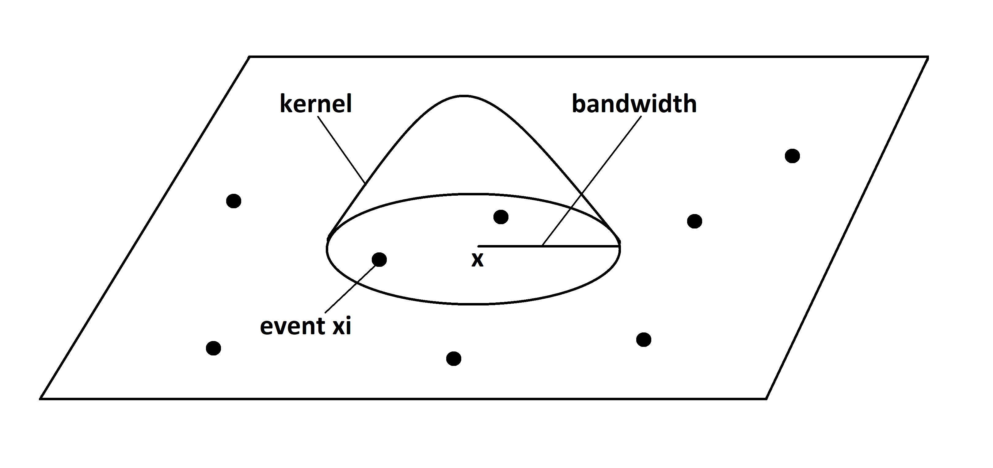
FIGURE 21.1: Kernel estimation representation.

21.1 Intensity

The density() function of spatstat can be used to obtain a kernel estimate of the intensity of a point pattern. The arguments of density() can be seen by typing ?density.ppp. These include the type of kernel (kernel) and the smoothing bandwidth (sigma). By default, density() uses a Gaussian kernel and a bandwidth determined by a simple rule of thumb that depends only on the size of the window. Here, we use the density() function to estimate the intensity of the point pattern of tree locations that is in the japanesepines data from spatstat (Figure 21.2).

library(spatstat)
X <- japanesepines
plot(X)
axis(1)
axis(2)

The density() function returns an intensity estimate object of class im that can be plotted (Figure 21.2). The kernel bandwidth used in density() can be extracted with the sigma attribute of the returned intensity object.

lambdahat <- density(X)
attr(lambdahat, "sigma")

[1] 0.125

Note that although the type kernel weakly influences the estimates, the bandwidth can have a big impact. For example, Figure 21.2 shows intensity estimates of the tree point pattern using different values of bandwidths. We observe that small values of the bandwidth result in estimated intensities that are too spiky, whereas large values provide smoother surfaces that may ignore local characteristics of the intensities.

plot(lambdahat, main = "Default bandwidth")
plot(density(X, sigma = 0.05))
plot(density(X, sigma = 0.1))
plot(density(X, sigma = 1))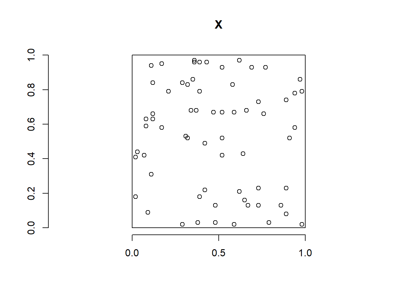

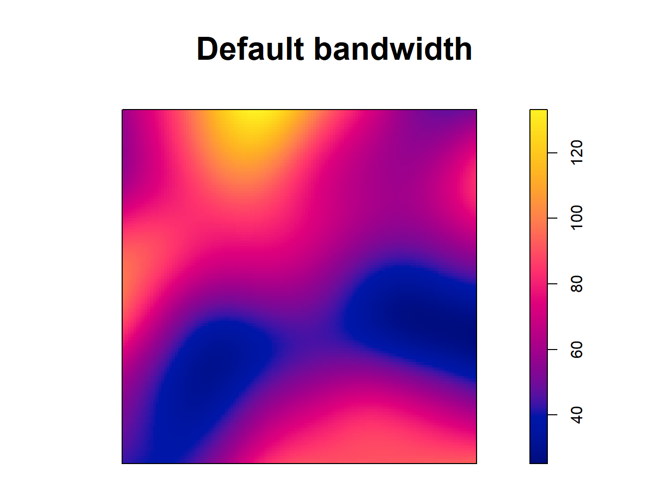
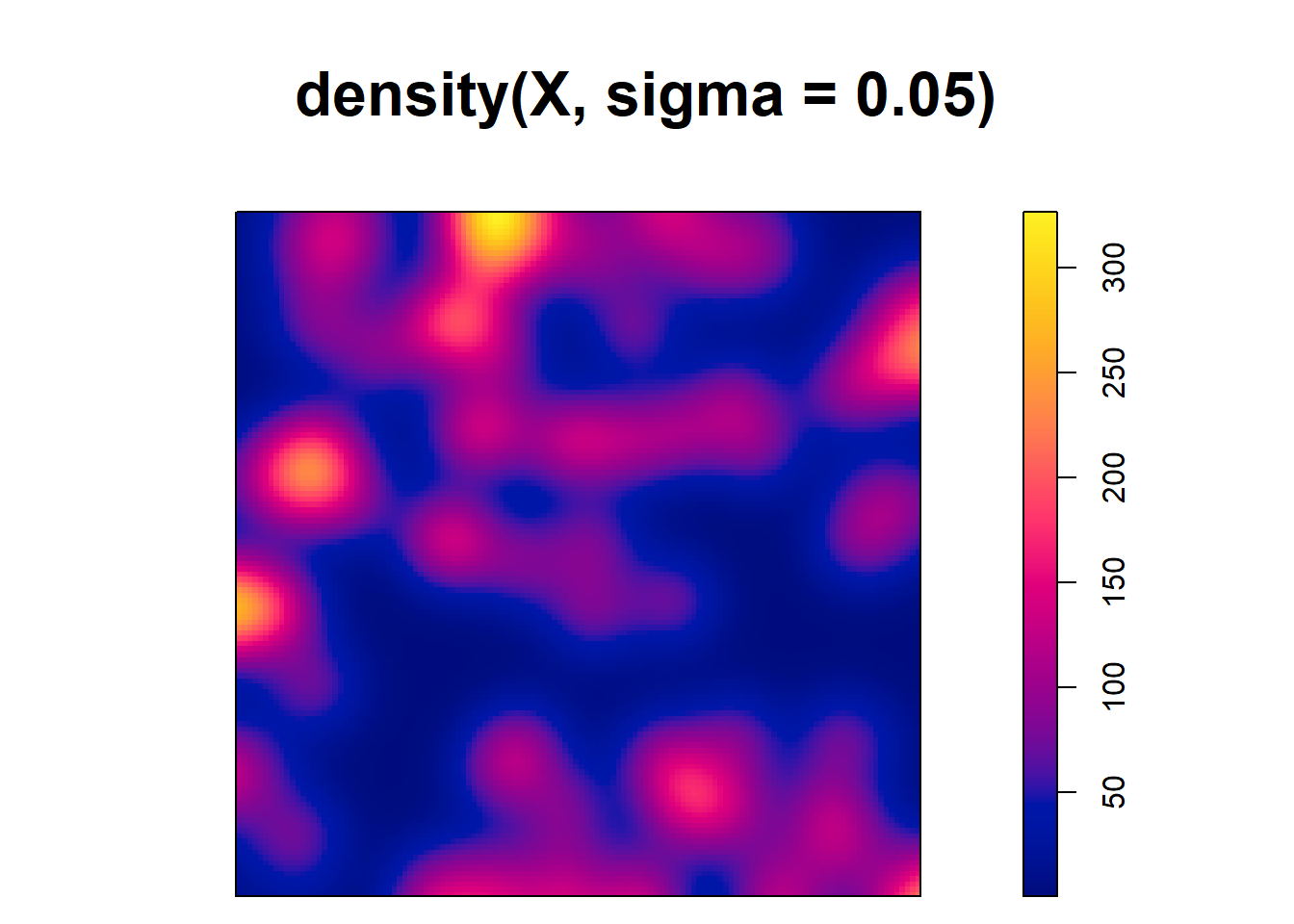
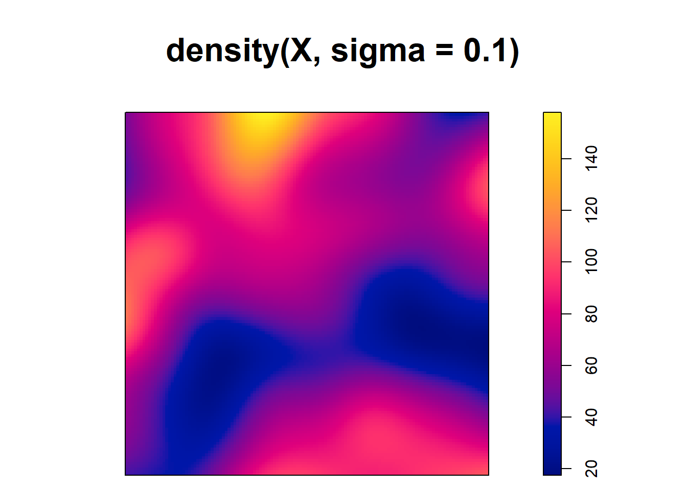
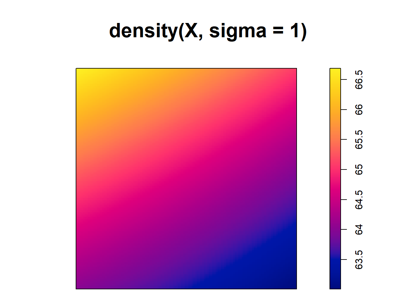
FIGURE 21.2: Top: Trees point pattern. Bottom: Intensity estimates using several values for the kernel bandwidth.

In practice, we may conduct exploratory analyses considering a number of possible bandwidth values to select, somewhat subjectively, an appropriate bandwidth. Other criteria such as cross-validation as implemented in the bw.diggle() and bw.ppl() functions of spatstat can be used to select a smoothing bandwidth for the kernel estimation of the point process intensity. We can also use adaptative kernel estimators where bandwidths change at each data point of the spatial point pattern (González and Moraga 2022, 2023c).

21.2 Intensity ratio

In some situations, we may want to compare two point patterns observed in the same region, such as the patterns of individuals with a disease, and set of controls representing at-risk population. We can do that by computing the intensity ratio of the patterns, which allows us to identify spatial patterns and hotspots in the relative risk surface obtained.

Here, we show how to estimate the intensity ratio of two point patterns using the density() function of spatstat, and we visualize the results with the image.plot() function of fields. Alternatively, we could estimate the intensity ratio by using the sparr package which provides functions to estimate and assess the significance of relative risk surfaces.

We consider the data pbc from the sparr package which contains 761 cases of primary biliary cirrhosis (PBC) along with 3020 controls representing at-risk population in north-eastern England collected between 1987 and 1994. This data is represented in Figure 21.3. The pbc data is a ppp object with marks case and control representing the cases and controls for the PBC data in north-eastern England. We create the ppp objects cases and controls with the events corresponding to each type.

library(sparr)
data(pbc)
cases <- unmark(pbc[which(pbc$marks == "case"), ])
plot(cases, main = "cases")
axis(1)
axis(2)
title(xlab = "Easting", ylab = "Northing")
controls <- unmark(pbc[which(pbc$marks == "control"), ])
plot(controls, pch = 3, main = "controls")
axis(1)
axis(2)
title(xlab = "Easting", ylab = "Northing")

library(sparr)
data(pbc)
cases <- unmark(pbc[which(pbc$marks == "case"), ])
controls <- unmark(pbc[which(pbc$marks == "control"), ])

We assume that the point pattern cases is a realization from a Poisson process with intensity \(\lambda(\boldsymbol{x})\), and that the point pattern controls come from a second, independent Poisson process with intensity \(\lambda_0(\boldsymbol{x})\). Then, we can express \(\lambda(\boldsymbol{x})\) as \[\lambda(\boldsymbol{x}) = \alpha \lambda_0(\boldsymbol{x}) \rho(\boldsymbol{x}).\]

Here, \(\rho(\boldsymbol{x})\) represents the spatial variation in relative risk. \(\alpha\) is a factor that adjusts the intensity estimate of the controls to take account that there are more controls than cases. This factor can be estimated as \(\hat \alpha = (\mbox{number of cases})/(\mbox{number of controls}).\) An estimate of the density ratio can then be obtained as the ratio of the kernel estimates of the intensity of cases and controls as follows:

\[\hat \rho(\boldsymbol{x}) = \frac{\hat \lambda(\boldsymbol{x})}{\hat \alpha \hat \lambda_0(\boldsymbol{x})}.\]

Here, we show how to compute and plot the relative risk for the PBC case-control data. First, we obtain a common bandwidth to obtain the kernel estimates of the intensities of cases and controls. We calculate this common bandwidth as the mean of the default bandwidths obtained when using density() to estimate the intensity of cases and controls separately.

bwcases <- attr(density(cases), "sigma")
bwcontr <- attr(density(controls), "sigma")
(bw <- (bwcases + bwcontr)/2)

[1] 11.46

Then, we use the selected bandwidth to compute the smoothed intensity estimates for the cases and controls.

intcases <- density(cases, sigma = bw)
intcontrols <- density(controls, sigma = bw)

We estimate \(\alpha\) as the ratio of the number of cases (cases$n = 761) to the number of controls (controls$n = 3020) to account for the fact that there are more controls than cases.

(alphahat <- cases$n/controls$n)

[1] 0.252

Then, using the intensity estimates of the cases and controls patterns, the relative risk is estimated as

\[\hat \rho(\boldsymbol{x}) = \frac{\hat \lambda(\boldsymbol{x})}{\hat \alpha \hat \lambda_0(\boldsymbol{x})}.\] Figure 21.3 shows the estimated intensity ratio obtained with the image.plot() function of the fields package. Note that to plot the intensity estimate object with image.plot(), we first need to transpose the image values returned by density() since they are stored in transposed form.

library(fields)
x <- intcases$xcol
y <- intcases$yrow
rr <- t(intcases$v)/t(alphahat * intcontrols$v)
image.plot(x, y, rr, asp = 1)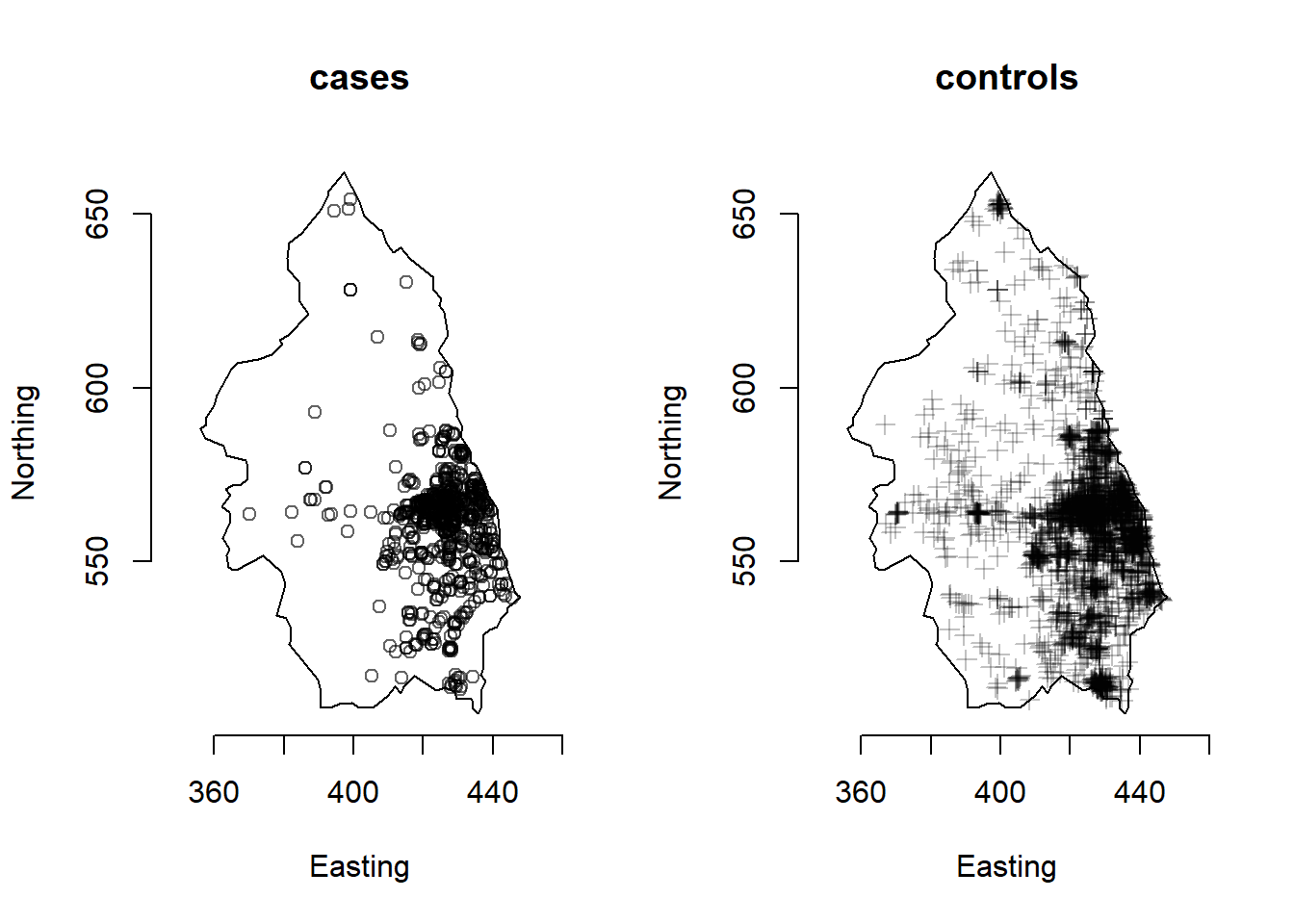

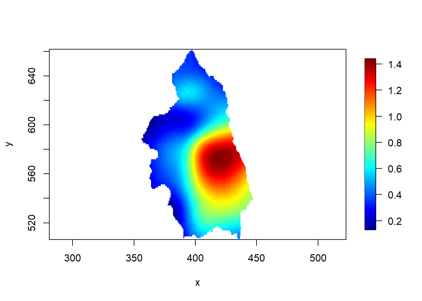
FIGURE 21.3: Cases of primary biliary cirrhosis and controls representing at-risk population (top) and intensity ratio (bottom) in north-eastern England between 1987 and 1994.

21.3 Intensity on networks

The spatstat package also contains functionality to work with spatial point patterns on linear networks. An example of this type of point pattern is given by the chicago data of spatstat. This data contains the locations and type of crimes reported from 25 April to 8 May 2002 in an area of Chicago, Illinois, USA. All crimes occurred on or near a street, and the data provide the coordinates of all streets in the survey area, and their connectivity. Spatial coordinates are expressed in feet (1 foot corresponds to 0.3048 meters). Figure 21.4 shows the crime locations by type and the streets of the study region.

library(spatstat)
X <- chicago
head(X$data)
X$domain
plot(X)

Hyperframe:
      x    y seg      tp   marks
1 639.2 1191  37 1.00000 assault
2 139.7 1135  54 0.36985 assault
3 195.3 1150  53 0.74153 assault
4 693.5 1125  72 0.02486 assault
5 596.4 1005 122 0.32558 assault
6 684.7 1005 124 0.90250 assault

Linear network with 338 vertices and 503 lines
Enclosing window: rectangle = [0.4, 1282] x [153.1, 
1276.6] feet

chicago is an object of class lpp (point pattern on a linear network). lpp objects contain the locations of the points as an ppp object or other object acceptable to as.ppp(), and a linear network of class linnet.

The density.lpp() function of spatstat allows us to obtain an estimate of the density of the events on the linear network by applying kernel smoothing. For example, Figure 21.4 shows the intensity of all types of crimes obtained using density.lpp() with a bandwidth of 10.

# unmarked point pattern
uX <- unmark(chicago)
# intensity estimate
lambdahat <- density.lpp(uX, sigma = 10)
# plot
plot(lambdahat, main = "Intensity")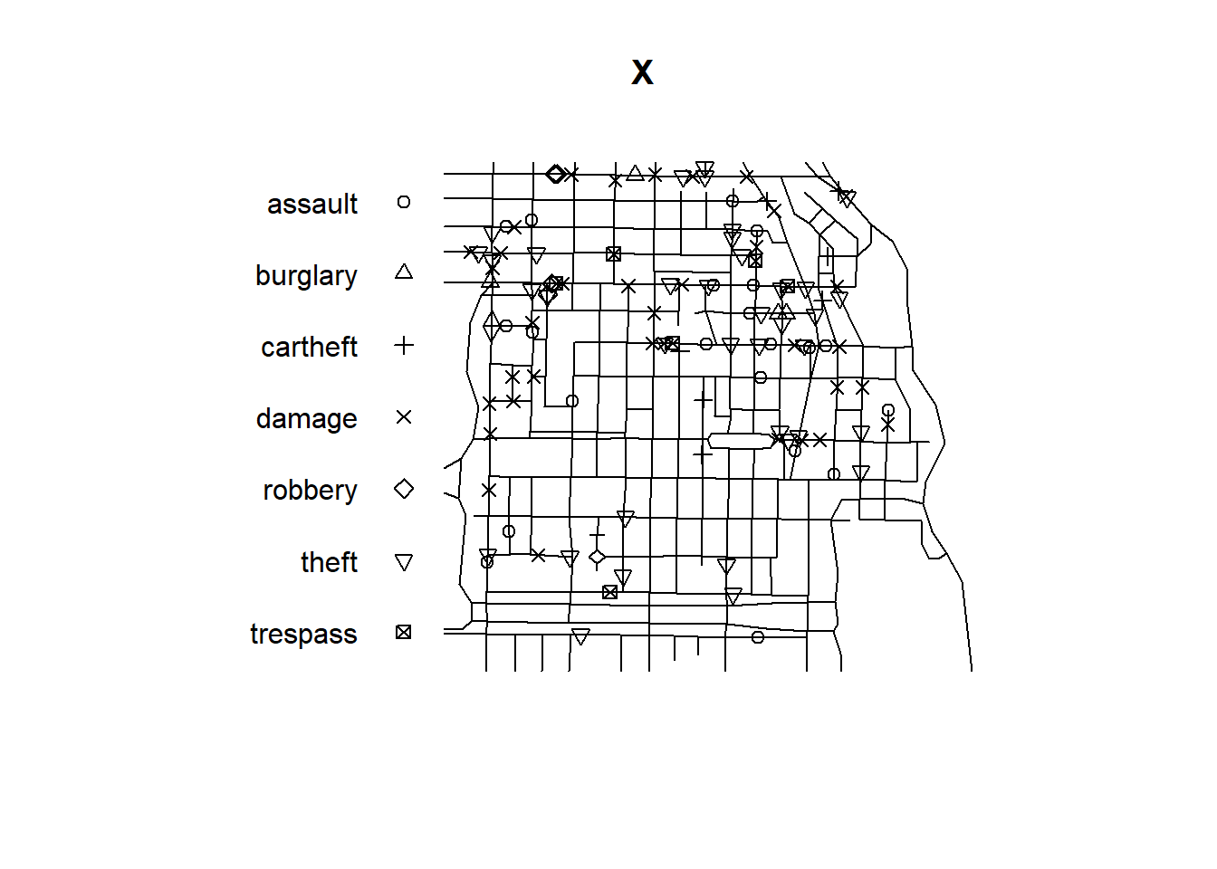

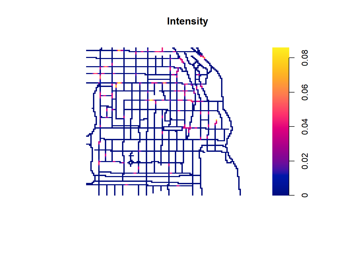
FIGURE 21.4: Crime locations by type (top) and intensity of crime locations (bottom) in an area of Chicago.