14 Kriging
Kriging (Matheron 1963) is a spatial interpolation method used to obtain predictions at unsampled locations based on observed geostatistical data. This method originated in the field of mining geology and is named after South African mining engineer Danie G. Krige. Suppose that we have observed data \(Z(\boldsymbol{s}_1), \ldots, Z(\boldsymbol{s}_n)\), and wish to predict the value of \(Z\) at an arbitrary location \(\boldsymbol{s}_0 \in D\). The Ordinary Kriging estimator of \(Z(\boldsymbol{s}_0)\) is defined as the linear unbiased estimator
\[\hat Z(\boldsymbol{s}_0) = \sum_{i=1}^n \lambda_i Z(\boldsymbol{s}_i)\] that minimizes the mean squared prediction error defined as
\[E[(\hat Z(\boldsymbol{s}_0)-Z(\boldsymbol{s}_0))^2].\]
The Kriging weights are derived from the estimated spatial structure of the sampled data. Specifically, weights are obtained by first fitting a variogram model to the observed data, which helps us understand how the correlation between observation values changes with the distance between locations. Once the Kriging weights are obtained, they are applied to the known data values at the sampled locations to calculate the predicted values at unsampled locations. The Kriging weights reflect the spatial correlation of the data, which accounts for the geographical proximity and similarity of data points. Thus, observed locations that are correlated and near to the prediction locations are given more weight than those uncorrelated and farther apart. Weights also take into account the spatial arrangement of all observations, so clusterings of observations in oversampled areas are weighted less heavily since they contain less information than single locations.
Under several assumptions, Kriging predictions are best linear unbiased estimators. There are several types of Kriging differing by underlying assumptions and analytic goals. For example, Simple Kriging assumes the mean of the random field, \(\mu(\boldsymbol{s})\), is known; Ordinary Kriging assumes a constant unknown mean, \(\mu(\boldsymbol{s}) = \mu\); and Universal Kriging can be used for data with an unknown non-stationary mean structure.
14.1 Kriging predictions of zinc concentrations
The gstat package (Pebesma and Graeler 2022) has functionality to model, predict, and simulate geostatistical data. Here, we provide an example on how to predict zinc concentrations using samples collected near the river Meuse, The Netherlands. First, we load the data and create maps with the sample and the prediction locations. Then, we show how to fit a model variogram to the empirical variogram, and we use this fit to obtain predictions using Kriging. Finally, we create maps of the predictions and their associated uncertainty.
14.1.1 Data
The meuse data from the sp package contains zinc and other soil-heavy metal concentrations collected at locations in a flood plain of the river Meuse near Stein, The Netherlands (Figure 14.1).
meuse.grid contains prediction grid locations for the meuse dataset (Figure 14.2).
We convert the meuse and meuse.grid data frames to sf objects using the st_as_sf() function and setting the coordinate reference system to EPSG 28992. We create maps using the mapview package.
library(sp)
library(gstat)
library(sf)
library(mapview)

data(meuse)
data(meuse.grid)

meuse <- st_as_sf(meuse, coords = c("x", "y"), crs = 28992)
mapview(meuse, zcol = "zinc",  map.types = "CartoDB.Voyager")

meuse.grid <- st_as_sf(meuse.grid, coords = c("x", "y"),
                       crs = 28992)
mapview(meuse.grid,  map.types = "CartoDB.Voyager")
FIGURE 14.1: Zinc concentrations at locations in a flood plain of the river Meuse.
FIGURE 14.2: Prediction locations.
14.1.2 Variogram cloud
The variogram cloud shows half of all possible squared differences of data observation pairs against their separation distance \(h\):
\[\frac{1}{2}(Z(\boldsymbol{s}) - Z(\boldsymbol{s}+h))^2\]
The variogram() function of gstat can be used to calculate the variogram cloud.
In variogram(), we set argument object to z ~ 1 if we wish to obtain the variogram for data z,
or to a formula of a linear model with covariates if we wish the variogram for the residuals.
Figure 14.3 shows the variogram cloud for the zinc data. This plot can be inspected to assess whether sample pairs closer to each other are more similar than pairs further apart.
14.1.3 Sample variogram
Assuming isotropy, the sample variogram averages the variogram cloud values over distance intervals:
\[2 \hat \gamma(h) = \frac{1}{|N(h)|} \sum_{N(h)} (Z(\boldsymbol{s}_i) - Z(\boldsymbol{s}_j))^2,\]
where \(|N(h)|\) denotes the number of distinct pairs in
\[N(h) = \{(\boldsymbol{s}_i, \boldsymbol{s}_j): ||\boldsymbol{s}_i-\boldsymbol{s}_j|| = h,\ i, j = 1, \ldots,n \}.\]
The variogram() function of gstat calculates the sample variogram from data or for residuals if a linear model has been specified.
We can also specify the argument
width indicating the width of distance intervals into which data point pairs are grouped to compute the estimates.
Figure 14.3 shows the sample variogram for the zinc data.
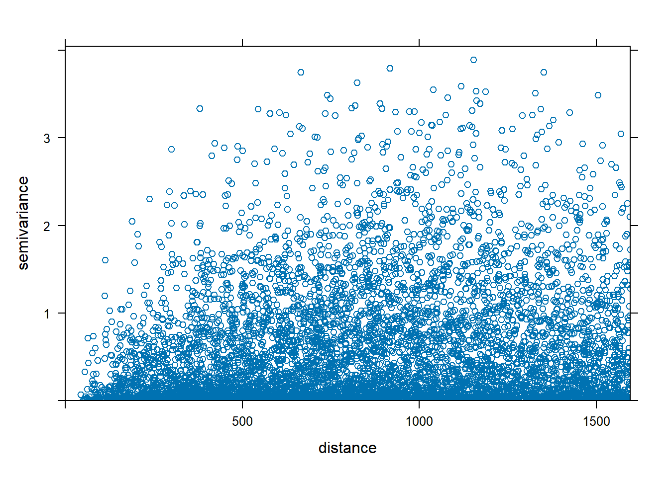
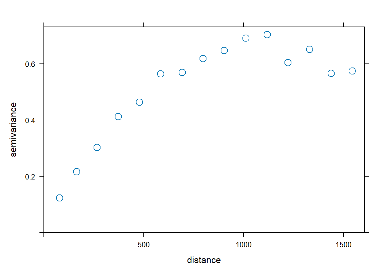
FIGURE 14.3: Variogram cloud (left) and sample variogram (right).
14.1.4 Fitted variogram
The sample variogram obtained is a function of distance \(h\) estimated at discrete lags (e.g., \(h(1), h(2),\ldots, h(k)\)). Then, we can fit a variogram model to these estimated values,
\[\{ \left(h(j),\ 2 \hat \gamma(h(j)) \right): j=1,2,\ldots,k\}.\]
The vgm() function of gstat generates a variogram model. This function has arguments model with the model type (e.g., Sph for spherical and Exp for exponential),
nugget, psill (partial sill, which is the sill minus the nugget) and range.
Details on the construction of the variogram models are given in Section 4.3 of the gstat user’s manual.
A list of available models can be printed with vgm() and visualized with show.vgms() (Figure 14.4).
vgm() short long
1 Nug Nug (nugget)
2 Exp Exp (exponential)
3 Sph Sph (spherical)
4 Gau Gau (gaussian)
5 Exc Exclass (Exponential class/stable)
6 Mat Mat (Matern)
7 Ste Mat (Matern, M. Stein's parameterization)
8 Cir Cir (circular)
9 Lin Lin (linear)
10 Bes Bes (bessel)
11 Pen Pen (pentaspherical)
12 Per Per (periodic)
13 Wav Wav (wave)
14 Hol Hol (hole)
15 Log Log (logarithmic)
16 Pow Pow (power)
17 Spl Spl (spline)
18 Leg Leg (Legendre)
19 Err Err (Measurement error)
20 Int Int (Intercept)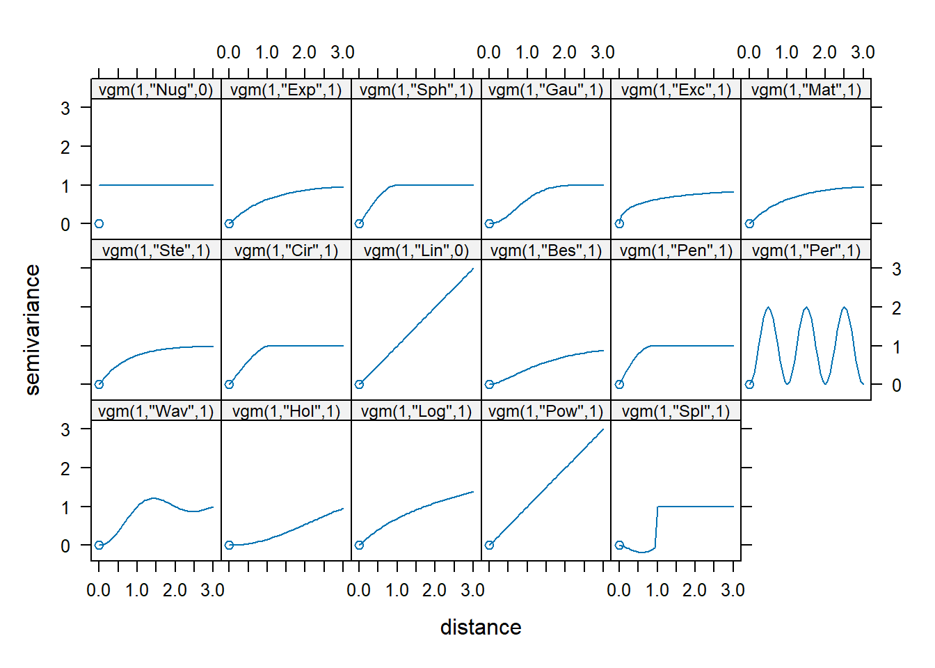
FIGURE 14.4: Available variogram models in gstat.
The fit.variogram() function fits a variogram model to a sample variogram.
Arguments of this function include object with the sample variogram, and model with the variogram model which is an output of vgm() with arguments nugget, psill, and range denoting initial values of the iterative fitting algorithm.
The fitting method is specified in fit.method and can be ordinary (unweighted) or weighted least squares using a weighting scheme that gives most weight to early lags and downweights those lags with a small number of pairs. Thus, if \(\{ 2 \gamma(h;\boldsymbol{\lambda})\}\) is a model depending on parameters \(\boldsymbol{\lambda}\), and \(w_j\) are weights associated to lag \(h(j)\), the method of weighted least squares chooses the value of \(\boldsymbol{\lambda}\) that minimizes
\[\sum_{j=1}^k w_j \left[2 \hat \gamma(h(j)) - 2 \gamma(h(j); \boldsymbol{\lambda})\right]^2.\]
By inspecting the sample variogram of the zinc data, we may think that a good model for the variogram would be spherical with initial values for the partial sill equal to 0.5, range equal to 900, and nugget equal to 0.1.
Figure 14.5 (left) shows the sample variogram v calculated with variogram(), and the variogram generated with vgm() using a spherical model, and with partial sill, range, and nugget equal to our initial guess values. This plot allows us to assess our initial model.
vinitial <- vgm(psill = 0.5, model = "Sph",
                range = 900, nugget = 0.1)
plot(v, vinitial, cutoff = 1000, cex = 1.5)
Then, we fit a variogram providing the sample variogram and choosing a spherical model (model = "Sph"), and the initial values for the partial sill, range, and the nugget for the iterative fitting algorithm. Figure 14.5 (right) shows the sample and the fitted variogram.
fv <- fit.variogram(object = v,
                    model = vgm(psill = 0.5, model = "Sph",
                                range = 900, nugget = 0.1))
fv
plot(v, fv, cex = 1.5)
model psill range
1 Nug 0.05066 0
2 Sph 0.59061 897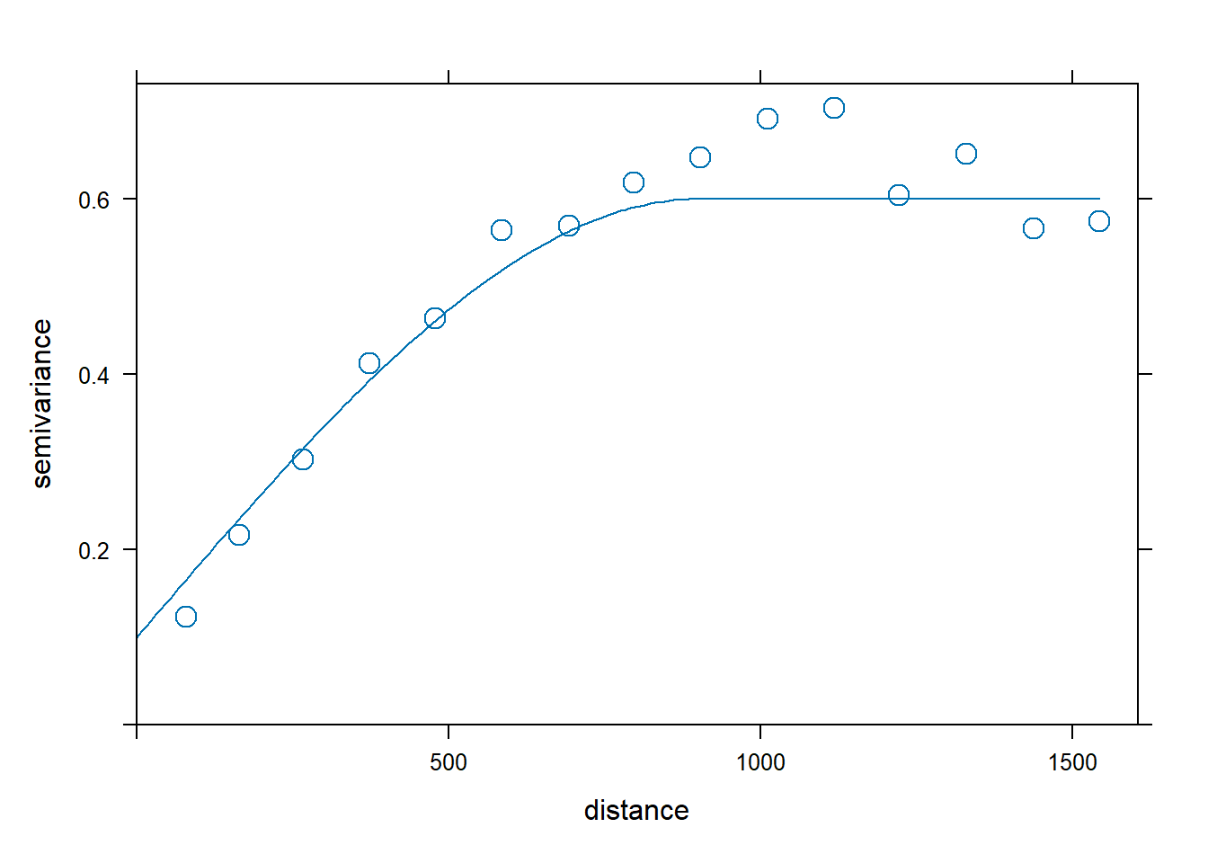
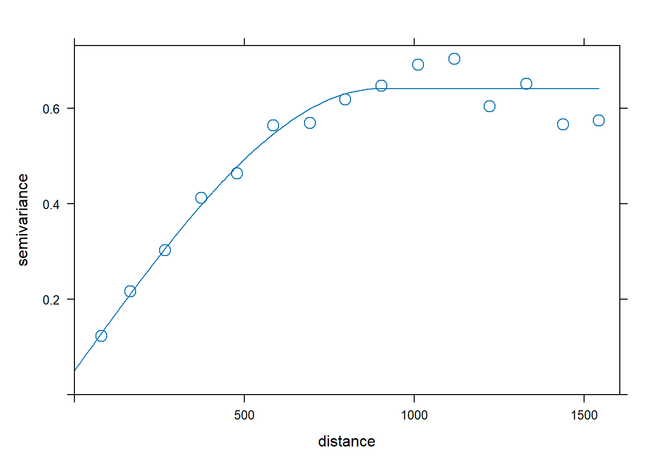
FIGURE 14.5: Sample variogram and variogram with initial parameters (left), and fitted model (right).
14.1.5 Kriging
Kriging uses the fitted variogram values fv to obtain predictions at unsampled locations.
Here, we use the gstat() function of gstat to compute the Kriging predictions.
Then, we obtain predictions at the unsampled locations given by meuse.grid with the predict.gstat() function.
kpred <- predict(k, meuse.grid)The returned object of predict() contains the predictions (var1.pred) and their variance (var1.var) which allow us to quantify the uncertainty of these predictions.
Figure 14.6 shows maps with the predictions and variance values.
Note that the Kriging predictions are calculated using weights that depend on the variogram estimates, and they are therefore sensitive to misspecification of the variogram model.
ggplot() + geom_sf(data = kpred, aes(color = var1.pred)) +
  geom_sf(data = meuse) +
  scale_color_viridis(name = "log(zinc)") + theme_bw()

ggplot() + geom_sf(data = kpred, aes(color = var1.var)) +
  geom_sf(data = meuse) +
  scale_color_viridis(name = "variance") + theme_bw()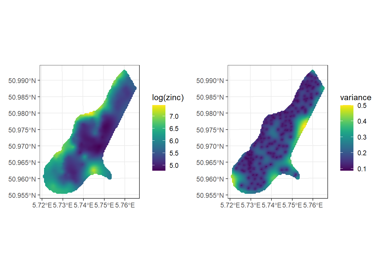
FIGURE 14.6: Predictions (left) and variance (right) obtained with Kriging.