22 The K-function

The K-function for a spatial point pattern \(\{\boldsymbol{x}_1, \ldots, \boldsymbol{x}_n\}\) observed in a planar window \(A \subset \mathbb{R^2}\), is an exploratory tool that can be used to assess the dependence between locations at several distances. The \(K\)-function is defined as

\[K(s) = \lambda^{-1}E[\mbox{number of further events within distance s of an arbitrary event}],\] where \(\lambda\) is the intensity function of the spatial point process.

For clustered spatial point patterns, each event is likely to be surrounded by further events. Therefore, for small values of the distance \(s\), \(K(s)\) will be relatively large. For regular point patterns, each event is likely to be surrounded by empty space. This implies that for small values of \(s\), \(K(s)\) will be relatively small.

To determine whether the values of a K-function are relatively large or small, we can compare the K-function for the observed spatial point pattern with the K-function for a homogeneous Poisson process (CSR) that is given by \(K(s) = \pi s^2\) as shown below. Thus, for a distance \(s\), \(K(s) > \pi s^2\) indicates clustering, and \(K(s) < \pi s^2\) suggests inhibition.

Let \(C\) be the region denoting the circle of center \(x_c\) and radius \(s\), and \(|C| = \pi s^2\) the area of the circle. Under complete spatial randomness (CSR), the intensity \(\lambda\) is constant equal to the observed number of events per unit area, and

\[E[\mbox{number of further events within distance s of an arbitrary event}] =\] \[ = \frac{\mbox{number of points in } C}{|C|} \times |C| = \lambda \times \pi s^2.\] Then, under CSR,

\[\lambda K(s) = E[\mbox{number of further events within distance s of an arbitrary event}] =\] \[ = \lambda \times \pi s^2,\]

which implies \(K(s) = \pi s^2\).

22.1 Estimating the K-function

Given a spatial point pattern \(\{\boldsymbol{x}_1, \ldots, \boldsymbol{x}_n\}\) in a planar window \(A\), we can construct an estimate of \(K(s)\) as follows. First, we define

\[E(s)= E[\mbox{number of further events within distance s of an arbitrary event}] =\] \[ = \lambda K(s).\] An estimate of \(E(s)\) can be computed as

\[\tilde E(s) = \frac{1}{n} \sum_{i=1}^n \sum_{j\neq i} I(d_{ij} \leq s),\] where \(d_{ij}\) is the distance between the events \(x_i\) and \(x_j\), and \(I(\cdot)\) is the indicator function (Figure 22.1).

The estimate \(\tilde E(s)\) is negatively biased because we do not observe events outside \(A\). This implies the observed counts for events \(x_i\) close to the boundary of \(A\) may be artificially low. To address this issue, we can introduce weights \(w_{ij}\) equal to the reciprocal of the proportion of the circle with center \(\boldsymbol{x}_i\) and radius \(d_{ij}\) which is contained in \(A\) (Figure 22.1). Then, an edge-corrected estimate for \(E(s)\) is given by

\[\hat E(s) = \frac{1}{n} \sum_{i=1}^n \sum_{j\neq i} w_{ij} I(d_{ij} \leq s).\]

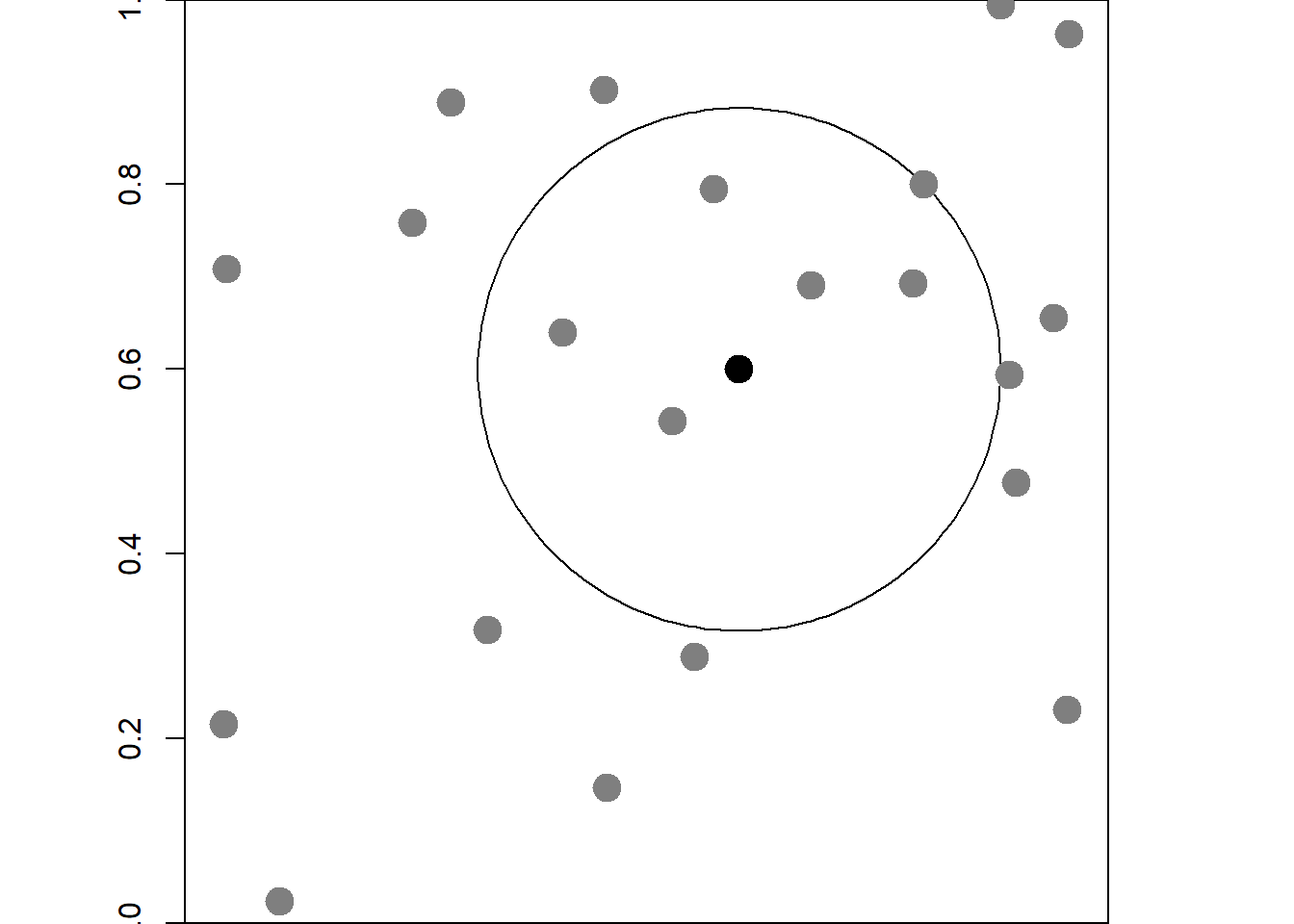
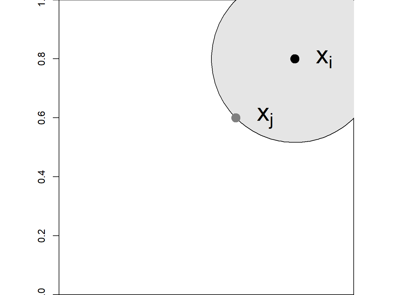
FIGURE 22.1: Left: Point pattern in the unit square region. The black point represents an arbitrary event. The circle encloses the events considered to estimate the K-function at the distance given by the radius of the circle. Right: Gray area represents the inverse of the weight used in the estimation of the K-function using the \(x_i\) and \(x_j\) events.

The intensity of a spatial point process denotes the expected number of events per unit area. In a homogeneous process, the intensity is constant and can be estimated as \(\hat \lambda = n/|A|\). Then, since \(K(s)=E(s)/\lambda\), the estimate of the K-function can be calculated as

\[\hat K(s) = \frac{ \hat E(s) }{\hat \lambda} = \frac{|A|}{n^2}\sum_{i=1}^n \sum_{j \neq i} w_{ij} I(d_{ij} \leq s).\]

22.2 The Kest() function

Given a spatial point pattern, the K-function can be estimated using the Kest() function of spatstat passing the spatial point pattern X as a ppp object or an object acceptable to as.ppp(). The Kest() function computes the K-function using three different edge-correction methods, namely, border, isotropic and translate, as well as the theoretical K-function for the homogeneous Poisson process.

Here, we use Kest() to estimate the K-function of a simulated spatial point pattern from a homogeneous Poisson process with intensity \(\lambda = 100\) in the region \([0, 1] \times [0, 1]\). Figure 22.2 shows the simulated point pattern with the rpoispp() function.

library(spatstat)
X <- rpoispp(lambda = 100)
plot(X)
axis(1)
axis(2)

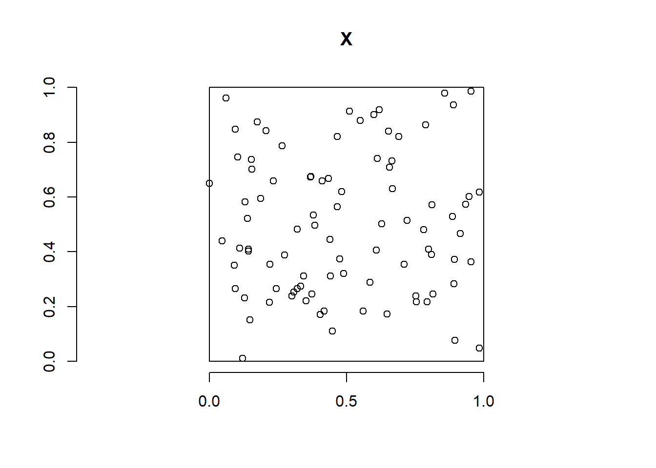
FIGURE 22.2: Simulated point pattern from a homogeneous Poisson process.

Figure ?? depicts the K-function calculated for this point pattern using different edge-correction methods together with the theoretical K-function for the homogeneous Poisson process.

K <- Kest(X)
plot(K)

The L-function is a commonly used function that transforms the K-function corresponding to a homogeneous Poisson process (\(K(s) = \pi s^2\)) to a straight line \(L(s) = s\) making visual interpretation easier. The L-function is defined as

\[L(s) = \sqrt{\frac{K(s)}{\pi}}.\]

The Lest() function can be used to estimate the \(L\)-function of a spatial point pattern. Figure ?? shows the L-functions for the simulated point pattern using different edge-correction methods, and the theoretical L-function for the homogeneous Poisson process.

L <- Lest(X)
plot(L)

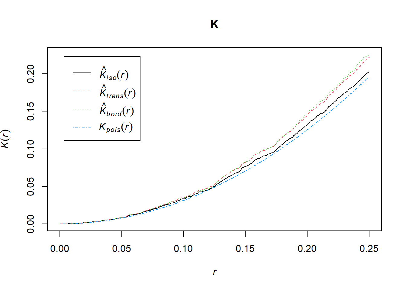
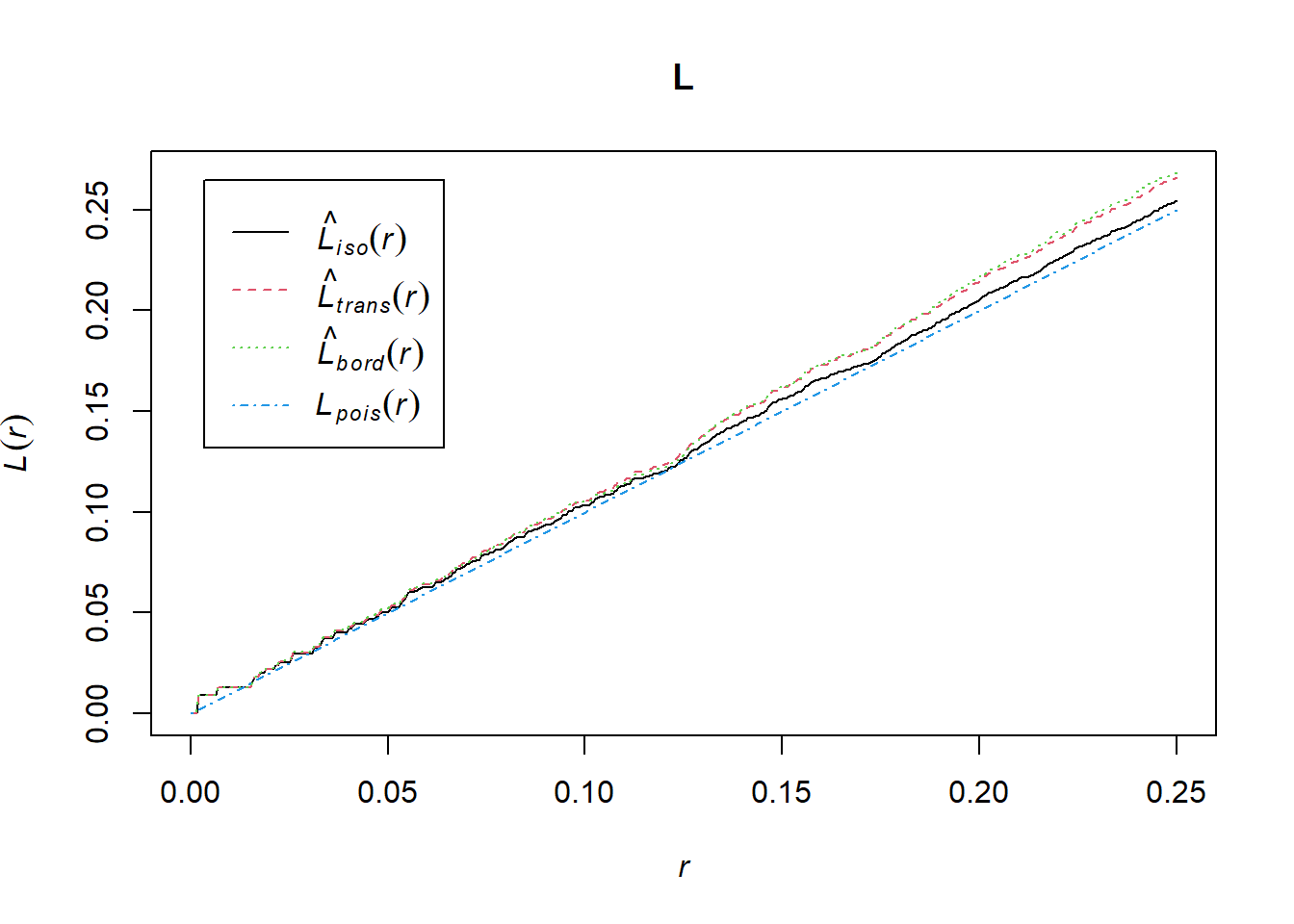
FIGURE 22.3: K-function (top) and L-function (bottom) corresponding to a simulated point pattern from a homogeneous Poisson process.

22.3 Testing complete spatial randomness

We can use the K-function to test complete spatial randomness (CSR) at a set of distances. Specifically, we can compare the K-function estimate from the data, \(\hat K(s)\), with the theoretical value of the K-function under CSR, (\(K(s) = \pi s^2\)). Typically, the estimated K-function does not lie exactly over the line \(\pi s^2\) representing the theoretical K-function under CSR. Therefore, to better assess CSR, we obtain a confidence region by simulating spatial point patterns under CSR. Then, we add the confidence region to the plot of the estimated K-function of the observed point pattern. This plot allows us to assess CSR by comparing the K-function corresponding to the observed data to the envelope for each of the distances. In more detail, we follow this approach:

• Generate a number of spatial point patterns (e.g., \(M = 99\), \(M = 999\)) of the same size as the observed pattern over the study region using a homogeneous Poisson process (CSR).
• For each spatial point pattern, estimate the K-function: \(\hat K_1(\cdot), \ldots, \hat K_M(\cdot)\).
• For each distance \(s\), compute the 95% quantile interval of \(\hat K_1(s), \ldots, \hat K_M(s)\).
• Reject the null hypothesis of CSR if the observed K-function at a given distance is outside the interval.

This approach can be conducted by using the envelope() function of spatstat which performs simulations and computes envelopes of a summary statistic based on the simulations. Specifically, envelope() generates nsim simulated point patterns each being a realization of a homogeneous Poisson point process (CSR) with the same intensity as the observed point pattern \(X\). Figure 22.4 shows the envelope obtained for 99 simulations under CSR. The confidence region obtained can be inspected to identify distances for which there is an indication of clustering or inhibition.

E <- envelope(X, Kest, nsim = 99)
plot(E)

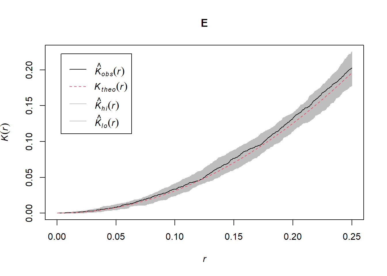
FIGURE 22.4: K-function of a simulated point pattern from a homogeneous Poisson process, together with an envelope corresponding to the K-functions of 99 simulated point patterns under CSR.