19 Spatial point processes and simulation

19.1 Spatial point processes

A stochastic process is a collection of random variables $X_i$ where $i$ belongs to an indexing set $I$, and each $X_i$ takes values in a sample space. A spatial point process $\{X_1, X_2, \ldots, X_{N(A)}\}$ is a stochastic process taking values in $A \subset \mathbb{R^2}$. A realization of a spatial point process is referred to as spatial point pattern and consists of a countable set of points $\{\boldsymbol{x}_1, \boldsymbol{x}_2, \ldots, \boldsymbol{x}_{N(A)}\}$ in the plane. We write $N(A)$ for the number of events in a planar region $A$, $N(A) = \# (\boldsymbol{x}_i \in A)$. Note that $N(A)$ is a random variable, and therefore, different realizations of the spatial point process may result in both different numbers and locations of events. We commonly refer to the points in the point pattern as events, to differentiate them from arbitrary points in the plane.

Let $d \boldsymbol{x}$ and $d \boldsymbol{y}$ denote small regions containing the points $\boldsymbol{x}$ and $\boldsymbol{y}$, respectively. The (first-order) intensity function of a spatial point process is defined as

\[\lambda(\boldsymbol{x}) = \lim_{|d\boldsymbol{x}| \rightarrow 0} \frac{E[N(d\boldsymbol{x})]}{|d\boldsymbol{x}|}.\]

The second-order intensity function is

\[\lambda_2(\boldsymbol{x}, \boldsymbol{y}) = \lim_{|d\boldsymbol{x}| \rightarrow 0, |d\boldsymbol{y}| \rightarrow 0} \frac{E[N(d\boldsymbol{x})N(d\boldsymbol{y})]}{|d\boldsymbol{x}||d\boldsymbol{y}|}.\]

The covariance density is expressed as

\[\gamma(\boldsymbol{x}, \boldsymbol{y}) = \lambda_2(\boldsymbol{x}, \boldsymbol{y})-\lambda(\boldsymbol{x})\lambda(\boldsymbol{y}).\]

A spatial point process is stationary and isotropic if its statistical properties do not change under translation and rotation, respectively. More specifically, for any integer $k$ and regions $\{A_i: i=1, \ldots, k\}$, a process is stationary if the joint distribution of $N(A_1),\ldots,N(A_k)$ is invariant to translation by an arbitrary amount $\boldsymbol{x}$. The process is isotropic if the joint distribution of $N(A_1),\ldots,N(A_k)$ is invariant to rotation through an arbitrary angle $\theta$. That is, if there are no directional effects. Moreover, the process is orderly if there can be no co-located observations so $\lim_{|A|\rightarrow 0}P(N(A)>1) = 0$.

Given a stationary and isotropic spatial point process, the intensity function is a constant equal to the expected number of events per unit area:

\[\lambda(\boldsymbol{x}) = \lambda = \frac{E[N(A)]}{|A|}.\]

Thus, the second-order intensity reduces to a function of distance:

\[\lambda_2(\boldsymbol{x}, \boldsymbol{y}) = \lambda_2(||\boldsymbol{x} - \boldsymbol{y}||)=\lambda_2(h),\]

where $h =||\boldsymbol{x}-\boldsymbol{y}||$ is the distance between $\boldsymbol{x}$ and $\boldsymbol{y}$. Moreover, the covariance density is expressed as

\[\gamma(\boldsymbol{x}, \boldsymbol{y}) =\gamma(h)=\lambda_2(h)-\lambda^2.\]

19.2 Poisson processes

Let $\lambda(\cdot)$ be a non-negative valued function, called intensity function of the spatial point process. A Poisson process is characterized by the following properties:

1. The number of events in any region $A$, $N(A)$, follows a Poisson distribution with mean

\[\mu(A) = \int_A \lambda(\boldsymbol{x}) d\boldsymbol{x}.\] Thus, $P(N(A) = n) = exp(-\mu(A))\frac{\mu(A)^n}{n!}$.

2. Given $N(A)=n$, the locations of the $n$ events in $A$ form an independent random sample from the distribution on $A$ with probability density function proportional to the intensity $\lambda(\cdot)$.

Poisson processes can be classified as homogeneous and inhomogeneous Poisson processes. In homogeneous Poisson processes, the intensity is constant ($\lambda(\boldsymbol{x}) = \lambda$, $\forall \boldsymbol{x}$), whereas in inhomogeneous Poisson processes, the intensity varies in space. Homogeneous Poisson processes are also referred to as complete spatial randomness (CSR). In CSR processes, the expected intensity of points is constant across any region, and there is no interaction between the points.

19.3 Simulating Poisson point patterns with `rpoispp()`

Simulating point patterns is useful when we want to test theoretical properties of the processes and compare them with the data we analyze. Here, we show how to use the rpoispp() function of the spatstat package to simulate spatial point patterns from homogeneous and inhomogeneous Poisson processes. The rpoispp() function accepts an argument lambda that indicates the intensity of the Poisson process. lambda can be a single positive number, function, or pixel image. The argument win of rpoispp() is the observation window in which to simulate the pattern. win can be an object of class owin or an object acceptable to as.owin().

19.3.1 Homogeneous point process

Here, we generate a spatial point pattern from a homogeneous Poisson process with intensity $\lambda = 100$ in the window $A = [0, 1] \times [0, 2]$ which has area $|A| = 2$. To do that, we use the rpoispp() function setting lambda = 100 and win to the observation window owin(xrange = c(0, 1), yrange = c(0, 2)). The generated point pattern is shown in Figure ??.

library(spatstat)
phom <- rpoispp(lambda = 100,
                win = owin(xrange = c(0, 1), yrange = c(0, 2)))
phom$n

[1] 201

plot(phom, main = "Homogeneous")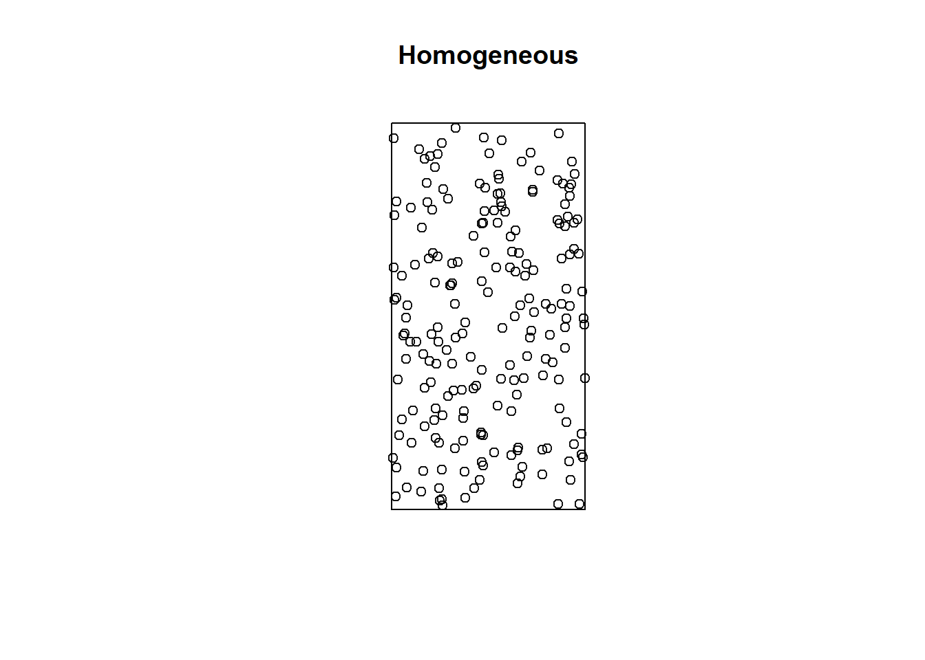

FIGURE 19.1: Point pattern generated from a homogeneous Poisson process.

Note that the difference between patterns generated with the rpoispp() and runifpoint() functions. rpoispp() generates a point pattern using an homogeneous Poisson process. In a homogeneous Poisson process, the generated number of points in a window $A$ follows a Poisson distribution with mean $\int_A \lambda(\boldsymbol{x}) d\boldsymbol{x} = \lambda \times |A|$ (expected number of points per unit area $\times$ area of the window), and the points are independent randomly distributed over the window. In our example, the number of points generated is equal to phom$n = 201. This number has been generated from a Poisson distribution with mean $\int_A \lambda(\boldsymbol{x}) d\boldsymbol{x} = \lambda \times |A| = 100 \times 2 = 200$. On the other hand, runifpoint() generates independent random points in the window conditioning on the total number of points equal to 200.

punif <- runifpoint(n = 200,
         win = owin(xrange = c(0, 1), yrange = c(0, 2)))
punif$n

[1] 200

19.3.2 Inhomogeneous point process

We can also use rpoispp() to generate a spatial point pattern from an inhomogeneous Poisson process. Here, we consider an intensity function $\lambda(x, y) = 10 + 100 \times x + 200 \times y$ and an observation window equal to $[0, 1] \times [0, 2]$. We write a function to evaluate the intensity function on a fine grid, and we visualize it to see how the intensity varies in space (Figure 19.2).

# intensity function
lambda <- function(x){return(10 + 100 * x[1] + 200 * x[2])}

# grid
xseq <- seq(0, 1, length.out = 50)
yseq <- seq(0, 2, length.out = 100)
grid <- expand.grid(xseq, yseq)

# evaluation of the function on a grid
z <- apply(grid, 1, lambda)

# plot
library(fields)
zmat <- matrix(z, 50, 100)
fields::image.plot(xseq, yseq, zmat, xlab = "x", ylab = "y",
                   main = "lambda(x, y)", asp = 1)

In point patterns generated from an inhomogeneous Poisson process, the number of events in any region follows a Poisson distribution with mean equal to the integral of the intensity over the region. Then, the location of each point is independently distributed in the region with probability density proportional to the intensity. In our example, the number of points is generated from a Poisson distribution with mean $\int_{[0, 1] \times [0,2]} \lambda(x,y) dx dy$ = 520. Figure 19.2 depicts the generated point pattern. We observe a higher number of points located in the regions where the intensity is higher.

fnintensity <- function(x, y){return(10 + 100 * x + 200 * y)}
pinhom <- rpoispp(lambda = fnintensity,
                  win = owin(xrange = c(0, 1), yrange = c(0, 2)))
pinhom$n
plot(pinhom, main = "Inhomogeneous")

[1] 532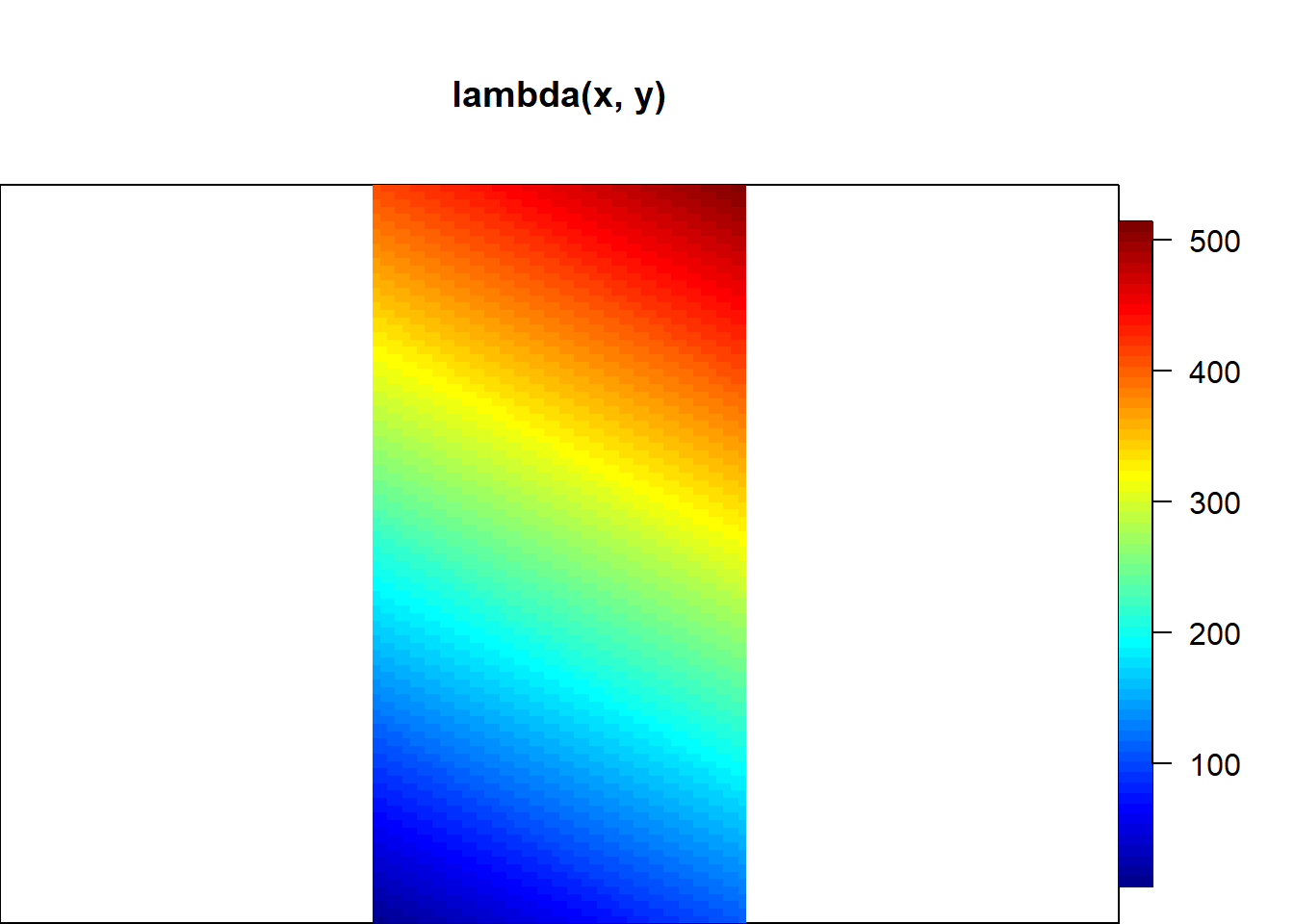

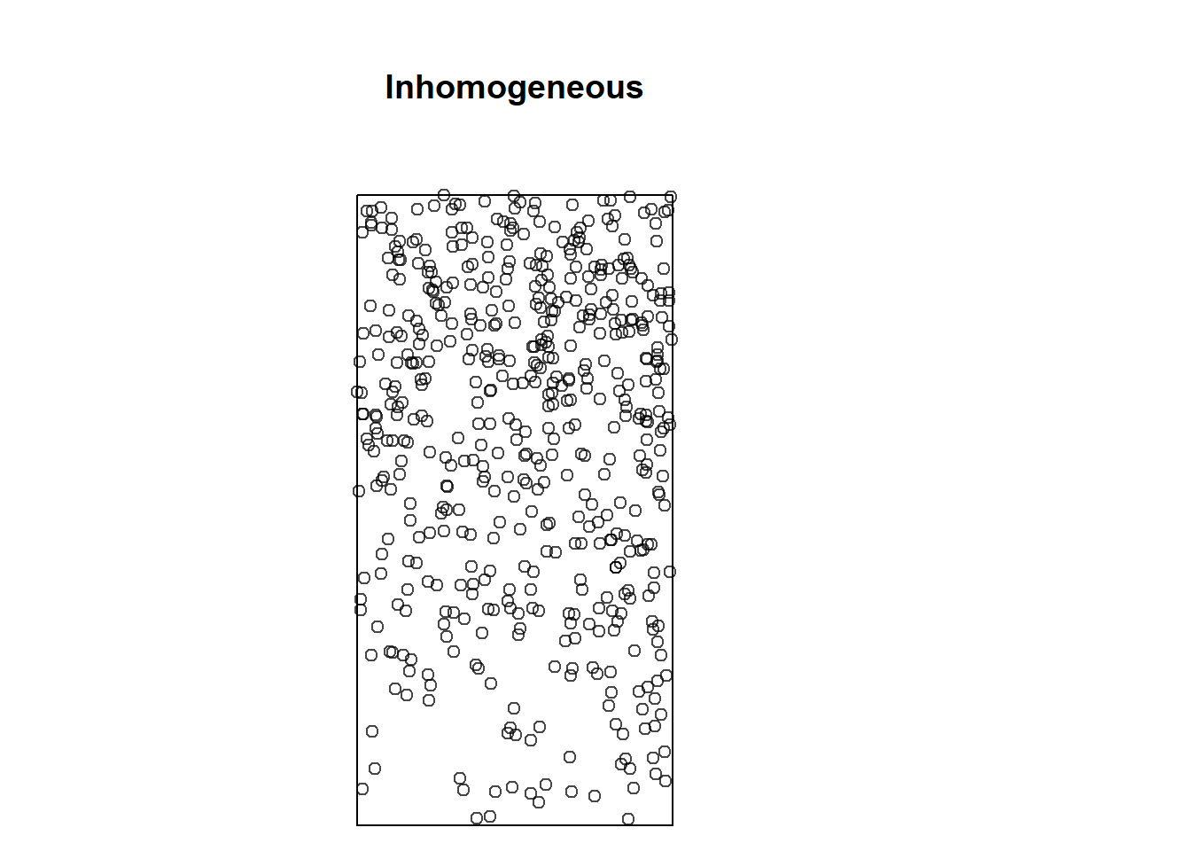
FIGURE 19.2: Intensity of an inhomogeneous Poisson process (top) and point pattern generated from that Poisson process (bottom).

18 The spatstat package

20 Complete spatial randomness