12 Geostatistical data

Geostatistical data provide information of a spatially continuous phenomenon that has been measured at particular sites. This type of data may represent, for example, air pollution levels taken at a set of monitoring stations or disease prevalence survey data at a collection of sites. Let \(Z(\boldsymbol{s}_1), \ldots, Z(\boldsymbol{s}_n)\) be observations of a spatial variable \(Z\) at locations \(\boldsymbol{s}_1, \ldots, \boldsymbol{s}_n\). In many situations, geostatistical data may be assumed to be a partial realization of a random process

\[\{Z(\boldsymbol{s}): \boldsymbol{s} \in D \subset \mathbb{R}^2 \},\]

where \(D\) is a fixed subset of \(\mathbb{R}^2\) and the spatial index \(\boldsymbol{s}\) varies continuously throughout \(D\). Often, for practical reasons, the process \(Z(\cdot)\) can only be observed at a finite set of locations. Based upon this partial realization, we may seek to infer the characteristics of the spatial process that gives rise to the data observed such as the mean and variability of the process. Then, we can use this information to predict the process at unsampled locations and construct a spatially continuous surface of the variable of study.

Kriging (Matheron 1963) and model-based geostatistics (Diggle, Tawn, and Moyeed 1998) are widely used approaches for spatial interpolation. Both approaches model the spatial distribution of the data to obtain predictions and their associated uncertainty at unsampled locations. Simpler spatial interpolation methods, such as the inverse distance weighted method, obtain predictions based on the spatial arrangement of the data. In the following chapters, we give an overview of Gaussian random fields. Then, we show how to employ spatial interpolation methods to obtain predictions using geostatistical data. We also show how to evaluate the predictive performance of the methods using a number of error measures and cross-validation.

12.1 Gaussian random fields

A Gaussian random field (GRF) \(\{Z(\boldsymbol{s}): \boldsymbol{s} \in D \subset \mathbb{R}^2 \}\) is a collection of random variables where observations occur in a continuous domain, and where every finite collection of random variables has a multivariate normal distribution. A random process \(Z(\cdot)\) is said to be strictly stationary if it is invariant to shifts. That is, if for any set of locations \(\boldsymbol{s}_i\), \(i=1,\ldots,n\), and any \(\boldsymbol{h} \in \mathbb{R}^2\) the distribution of \(\{Z(\boldsymbol{s}_1), \ldots, Z(\boldsymbol{s}_n)\}\) is the same as that of \(\{Z(\boldsymbol{s}_1 + \boldsymbol{h}), \ldots, Z(\boldsymbol{s}_n + \boldsymbol{h})\}\). A less restrictive condition is given by the second-order stationarity (or weakly stationarity). Under this condition, the process has constant mean,

\[E[Z(\boldsymbol{s})] = \mu, \forall \boldsymbol{s} \in D,\] and the covariances depend only on the differences between locations,

\[Cov( Z(\boldsymbol{s}), Z(\boldsymbol{s}+\boldsymbol{h})) = C(\boldsymbol{h}), \forall \boldsymbol{s} \in D, \forall \boldsymbol{h} \in \mathbb{R}^2.\]

In addition, if the covariances are functions only of the distances between locations \(h=||\boldsymbol{h}||\) and not of the directions, the process is called isotropic. If not, it is anisotropic. A process is said to be intrinsically stationary if, in addition to the constant mean assumption, it satisfies

\[Var[Z(\boldsymbol{s}_i) - Z(\boldsymbol{s}_j)] = 2 \gamma (\boldsymbol{s}_i - \boldsymbol{s}_j), \forall \boldsymbol{s}_i, \boldsymbol{s}_j.\]

12.2 Covariance functions of Gaussian random fields

Given a stationary and isotropic Gaussian random process \(Z(\cdot)\), the covariance function between a pair of variables separated by a distance \(h\) can be expressed as \[C(h) = \sigma^2 \mbox{Corr}(h),\] where \(\sigma^2\) denotes the variance of the spatial field, and \(\{\mbox{Corr}(h): h\in \mathbb{R}\}\) is a positive definite correlation function.

The Matérn family represents a very flexible class of correlation functions that appears naturally in many scientific fields. This family can be specified as

\[\mbox{Corr}(h) = \frac{1}{2^{\nu-1} \Gamma(\nu)} \left(\frac{h}{\phi}\right)^{\nu} K_{\nu}\left(\frac{h}{\phi}\right),\]

where \(h\) denotes the distance between locations, and \(K_\nu(\cdot)\) is the modified Bessel function of second kind and order \(\nu>0\). The parameter \(\phi >0\) controls how fast the correlation decays with distance and is related to the range, the distance at which the correlation between two points is approximately 0. The parameter \(\nu\) determines the smoothness of the process. This parameter is difficult to estimate in applications, and it is usually fixed to reflect scientific knowledge about the smoothness of the process \(Z(\cdot)\) (Diggle and Ribeiro Jr. 2007).

Special classes of the Matérn family include the exponential correlation function \(\mbox{Corr}(h) = exp(-h/\phi)\) when \(\nu = 0.5\), and the squared exponential or Gaussian correlation function \(\mbox{Corr}(h) = exp( - (h/\phi)^2 )\) when \(\nu \rightarrow \infty\).

12.3 Simulating Gaussian random fields

Here, we show how to generate realizations of several Gaussian random fields using the geoR package (Ribeiro Jr et al. 2022). Other packages that can be used to simulate Gaussian random fields include RandomFields (Schlather et al. 2015) and gstat (Pebesma and Graeler 2022).

The cov.spatial() function of geoR computes the value of the covariance function \(C(h) = \sigma^2 \mbox{Corr}(h)\) between a pair of variables located at points separated by distance \(h\), where \(\sigma^2\) is the variance parameter and \(\mbox{Corr}(h)\) is a positive definite correlation function. The types of covariance functions implemented in geoR can be seen by typing ?cov.spatial.

The grf() function of geoR can be used to simulate realizations of a Gaussian random field by specifying the following arguments:

• n is the number of points in the simulation. Here, we choose 1024 to simulate in a grid with 32 \(\times\) 32 cells.
• grid can be set to "reg" to simulate in a regular grid or "irreg" to simulate in a number of coordinates.
• xlims and ylims specify the limits of the area in the x and y directions, respectively. Here, we generate the field in a squared region \([0, 1] \times [0, 1]\) by using the default values xlims = c(0, 1) and ylims = c(0, 1).
• cov.model denotes the type of correlation function (e.g., "matern"). Possible types are detailed in the cov.spatial() function.
• cov.pars specifies the covariance parameters that indicate the variance \(\sigma^2\) and the parameter related to the range \(\phi\).
• kappa is the smoothness parameter required by some correlation functions such as "matern". By default, kappa = 0.5. In particular, kappa represents \(\nu\) in the definition of the Matérn function above.

Here, we show the correlation functions and realizations of Gaussian random fields with Matérn covariance function,

\[\mbox{C}(h) = \frac{\sigma^2}{2^{\nu-1} \Gamma(\nu)} \left(\frac{h}{\phi}\right)^{\nu} K_{\nu}\left(\frac{h}{\phi}\right),\]

with \(\sigma^2 = 1\) and \(\phi =\) 0.01, 0.2 and 1 to show different patterns of spatial variability. Figure 12.1 shows the covariance functions and realizations corresponding to each of the Gaussian random fields. We observe the correlation goes to 0 with distance, and it goes faster to 0 with smaller values of \(\phi\). The realizations of Gaussian random fields show less spatial autocorrelation for smaller values of \(\phi\).

covmodel <- "matern"
sigma2 <- 1

# Plot covariance function
curve(cov.spatial(x, cov.pars = c(sigma2, 1),
                  cov.model = covmodel), lty = 1,
      from = 0, to = 1, ylim = c(0, 1), main = "Matérn",
      xlab = "distance", ylab = "Covariance(distance)")
curve(cov.spatial(x, cov.pars = c(sigma2, 0.2),
                  cov.model = covmodel), lty = 2, add = TRUE)
curve(cov.spatial(x, cov.pars = c(sigma2, 0.01),
                  cov.model = covmodel), lty = 3, add = TRUE)

legend(cex = 1.5, "topright", lty = c(1, 1, 2, 3),
       col = c("white", "black", "black", "black"),
       lwd = 2, bty = "n", inset = .01,
       c(expression(paste(sigma^2, " = 1 ")),
         expression(paste(phi, " = 1")),
         expression(paste(phi, " = 0.2")),
         expression(paste(phi, " = 0.01"))))

# Simulate Gaussian random field in a regular grid 32 X 32
sim1 <- grf(1024, grid = "reg",
            cov.model = covmodel, cov.pars = c(sigma2, 1))
sim2 <- grf(1024, grid = "reg",
            cov.model = covmodel, cov.pars = c(sigma2, 0.2))
sim3 <- grf(1024, grid = "reg",
            cov.model = covmodel, cov.pars = c(sigma2, 0.01))

# Plot Gaussian random field
par(mfrow = c(1, 3), mar = c(2, 2, 2, 0.2))
image(sim1, main = expression(paste(phi, " = 1")), cex.main = 2,
      col = gray(seq(1, 0.1, l = 30)), xlab = "", ylab = "")
image(sim2, main = expression(paste(phi, " = 0.2")), cex.main = 2,
      col = gray(seq(1, 0.1, l = 30)), xlab = "", ylab = "")
image(sim3, main = expression(paste(phi, " = 0.01")), cex.main=2,
      col = gray(seq(1, 0.1, l = 30)), xlab = "", ylab = "")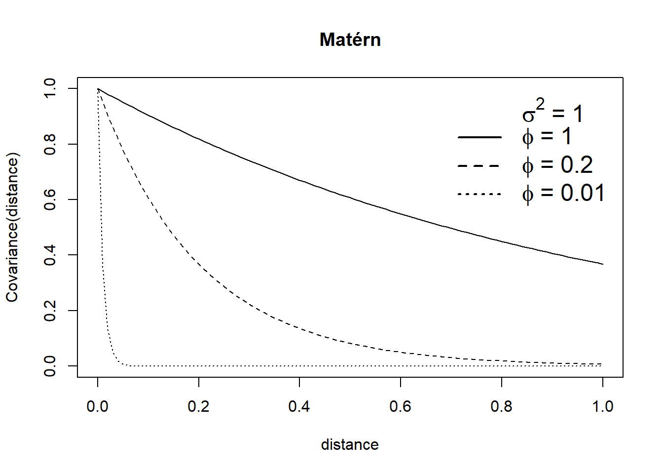

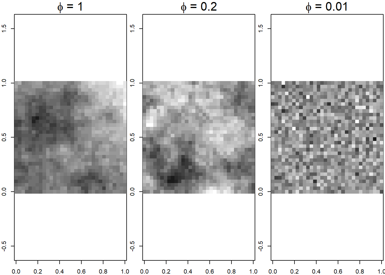
FIGURE 12.1: Covariance functions (top) and realizations of Gaussian random fields (bottom) for several parameter values.

12.4 Variogram

We can summarize the covariance structure of a spatial Gaussian random field with its variogram \(2 \gamma(\cdot)\) (or semivariogram \(\gamma(\cdot)\)). The variogram of a Gaussian random field \(Z(\cdot)\) is defined as the function

\[Var[Z(\boldsymbol{s}_i) - Z(\boldsymbol{s}_j)] = 2 \gamma (\boldsymbol{s}_i - \boldsymbol{s}_j).\]

Under the assumption of intrinsic stationarity, the constant-mean assumption implies

\[2 \gamma(\boldsymbol{h}) = Var(Z(\boldsymbol{s}+\boldsymbol{h}) - Z(\boldsymbol{s})) = E[(Z(\boldsymbol{s}+\boldsymbol{h}) - Z(\boldsymbol{s}))^2],\] and the semivariogram can be easily estimated with the empirical semivariogram as follows:

\[2 \hat \gamma(\boldsymbol{h}) = \frac{1}{|N(\boldsymbol{h})|} \sum_{N(\boldsymbol{h})} (Z(\boldsymbol{s}_i) - Z(\boldsymbol{s}_j))^2,\] where \(|N(\boldsymbol{h})|\) denotes the number of distinct pairs in \(N(\boldsymbol{h}) = \{(\boldsymbol{s}_i, \boldsymbol{s}_j): \boldsymbol{s}_i-\boldsymbol{s}_j = \boldsymbol{h},\ i, j = 1, \ldots,n \}\). Note that if the process is isotropic, the semivariogram is a function of the distance \(h=||\boldsymbol{h}||\).

The empirical semivariogram, when plotted against the separation distance, provides crucial insights into the continuity and spatial variability of the process. Figure 12.2 shows a plot of a typical semivariogram. Often, at shorter distances, the semivariogram tends to be small, indicating a higher similarity among observations in close proximity compared to those farther apart. As the separation distance increases, the semivariogram tends to increase as well, suggesting a decrease in similarity between observations with increasing distance.

Beyond a certain separation distance known as the range, the semivariogram levels off and reaches a nearly constant value referred to as the sill. This indicates that spatial dependence between observations decays with distance within the range, and beyond that range, observations become spatially uncorrelated, resulting in a near constant variance.

If there is a discontinuity or vertical jump at the origin of the plot, it signifies a nugget effect in the process. This effect is often attributed to measurement error but can also indicate a spatially discontinuous process.

The empirical semivariogram serves as a valuable exploratory tool for evaluating the presence of spatial correlation in data. Additionally, we can compare the empirical semivariogram to a Monte Carlo envelope constructed by computing empirical semivariograms from random permutations of the data while keeping the locations fixed. If the empirical semivariogram shows an increasing trend with distance and lies outside the Monte Carlo envelope, it provides evidence of spatial correlation.

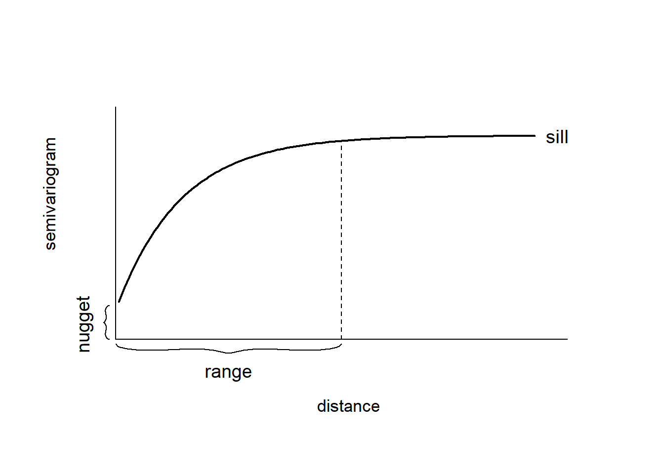
FIGURE 12.2: Typical semivariogram.

Example

Here, we show how to estimate the variogram function of geostatistical data using the variog() function of geoR. We use the parana data from geoR which contains the average rainfall over different years for the period May to June at 123 monitoring stations in Paraná state, Brazil. We use the st_as_sf() package to create a sf object with the rainfall data and create a map depicting the rainfall values with ggplot2 (Figure 12.3).

library(geoR)
library(ggplot2)
library(sf)
d <- st_as_sf(data.frame(x = parana$coords[, 1],
                         y = parana$coords[, 2],
                         value = parana$data),
              coords = c("x", "y"))

ggplot(d) + geom_sf(aes(color = value), size = 2) +
scale_color_gradient(low = "blue", high = "orange") +
geom_path(data = data.frame(parana$border), aes(east, north)) +
theme_bw()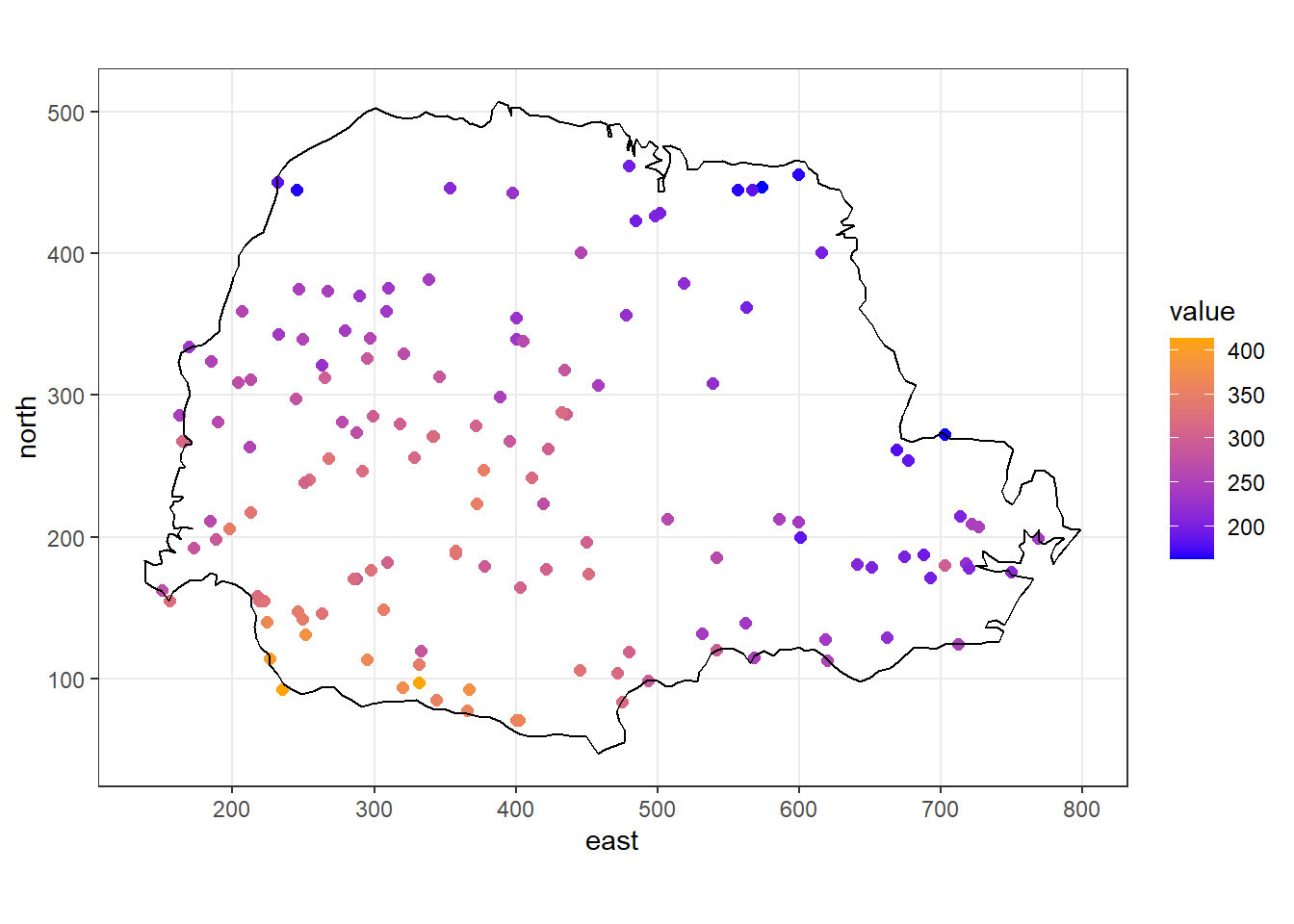

FIGURE 12.3: Rainfall values measured at 143 recording stations in Paraná state, Brazil.

In variog(), the argument option specifies the type of variogram. Possible values of option are binned ("bin"), cloud ("cloud"), and kernel smoothed variogram ("smooth"). The variogram cloud of a set of geostatistical data is a scatterplot of the points \((h_{ij}, v_{ij})\) defined as \(h_{ij} = ||\boldsymbol{s}_i - \boldsymbol{s}_j||\) and \(v_{ij} = \frac{1}{2} (Z(\boldsymbol{s}_i) - Z(\boldsymbol{s}_j))^2\).

When the underlying process has a spatially varying mean \(\mu(\boldsymbol{s})\), we compute \(v_{ij}\) using the residuals \(\left( Z(\boldsymbol{s}_i) - \hat \mu(\boldsymbol{s}_i) \right)\) instead of the data \(Z(\boldsymbol{s}_i)\). Argument trend of variog() denotes the trend fitted using ordinary least squares so variograms are computed using the residuals. By default, trend = "cte" so the mean is assumed constant over the region.

Figure 12.4 shows the empirical variogram corresponding to the rainfall data in Paraná state. It also shows the empirical variogram obtained by averaging values \(v_{ij}\)’s for which \(|h - h_{ij}| < u/2\), where \(u\) is a chosen bandwidth.

plot(variog(coords = st_coordinates(d), data = d$value,
            option = "cloud", max.dist = 400))

plot(variog(parana, max.dist = 400))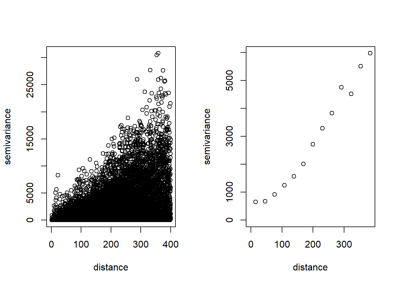

FIGURE 12.4: Empirical variogram values (left) and averaged empirical variogram values (right) corresponding to the rainfall data in Paraná state, Brazil.

The covariance parameters can be estimated by fitting a parametric covariance function to the empirical variogram. We can obtain the estimates by eye without a formal criterion, or by using ordinary or weighted least squares methods as we will see in the next chapters.