17 Spatial point patterns
Spatial point patterns are countable sets of points that arise as realizations of stochastic spatial point processes taking values in a planar region \(A \subset \mathbb{R^2}\). A spatial point pattern can be denoted as \(\{\boldsymbol{x}_1, \boldsymbol{x}_2, \ldots, \boldsymbol{x}_{N(A)}\}\), where \(N(A)\) is the number of points in \(A\). Note that \(N(A)\) is a random variable. Therefore, different realizations of the spatial point process may result in both different numbers and locations of points (Baddeley, Rubak, and Turner 2016). We often refer to the points in the point pattern as events to distinguish them from arbitrary points in the plane.
Spatial point patterns arise in many domains. Examples include locations of individuals with a certain disease in a city (Moraga and Montes 2011; Ribeiro Amaral, González, and Moraga 2023), species in a region (Moraga 2021b), and cells in a tissue (González and Moraga 2023a). The spatstat package (Baddeley, Turner, and Rubak 2022) can be used to work with spatial point patterns. The package includes a number of functions that allow us to conduct spatial analysis, such as assessing the randomness of spatial point patterns, and to formulate and fit models to point pattern data.
An example of spatial point pattern is given by the swedishpines data from spatstat. This pattern represents the locations of 71 trees in a Swedish forest plot of 9.6 \(\times\) 10 meters (Figure 17.1).
To get an impression of the spatial point pattern, we can calculate the intensity of events, which indicates the mean number of events per unit area.
The density() function of the spatstat package can be used to compute a kernel smoothed intensity function from a point pattern.
This function has an argument called kernel that indicates the type of kernel (Gaussian by default), and an argument called sigma which refers to the smoothing bandwidth, the standard deviation of the smoothing kernel.
In the swedishpines data, the coordinates of the point pattern are expressed in decimeters (0.1 meter).
Here, we use density() with sigma = 10 so the smoothing bandwidth is 10 decimeters or 1 meter.
Figure 17.1 shows the estimated intensity.
We observe that the intensity varies across the region, and
the average intensity is equal to 0.0074 trees per square decimeter, that is, 0.74 trees per square meter.
# density() calls density.ppp() if the argument is a ppp object
den <- density(x = X, sigma = 10)
summary(den)
plot(den, main = "Intensity")
contour(den, add = TRUE) # contour plot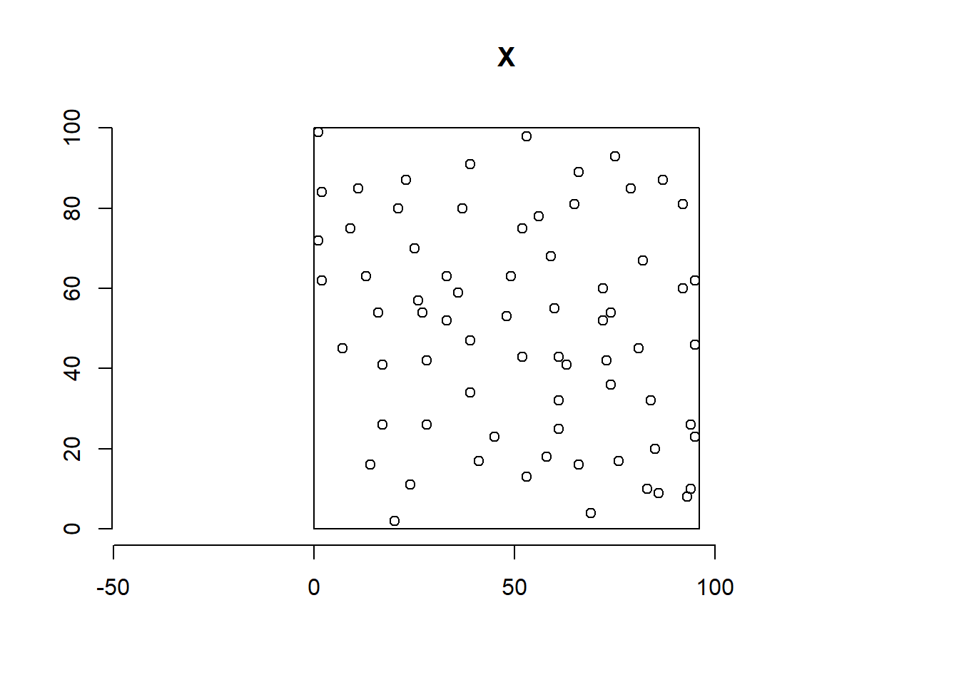
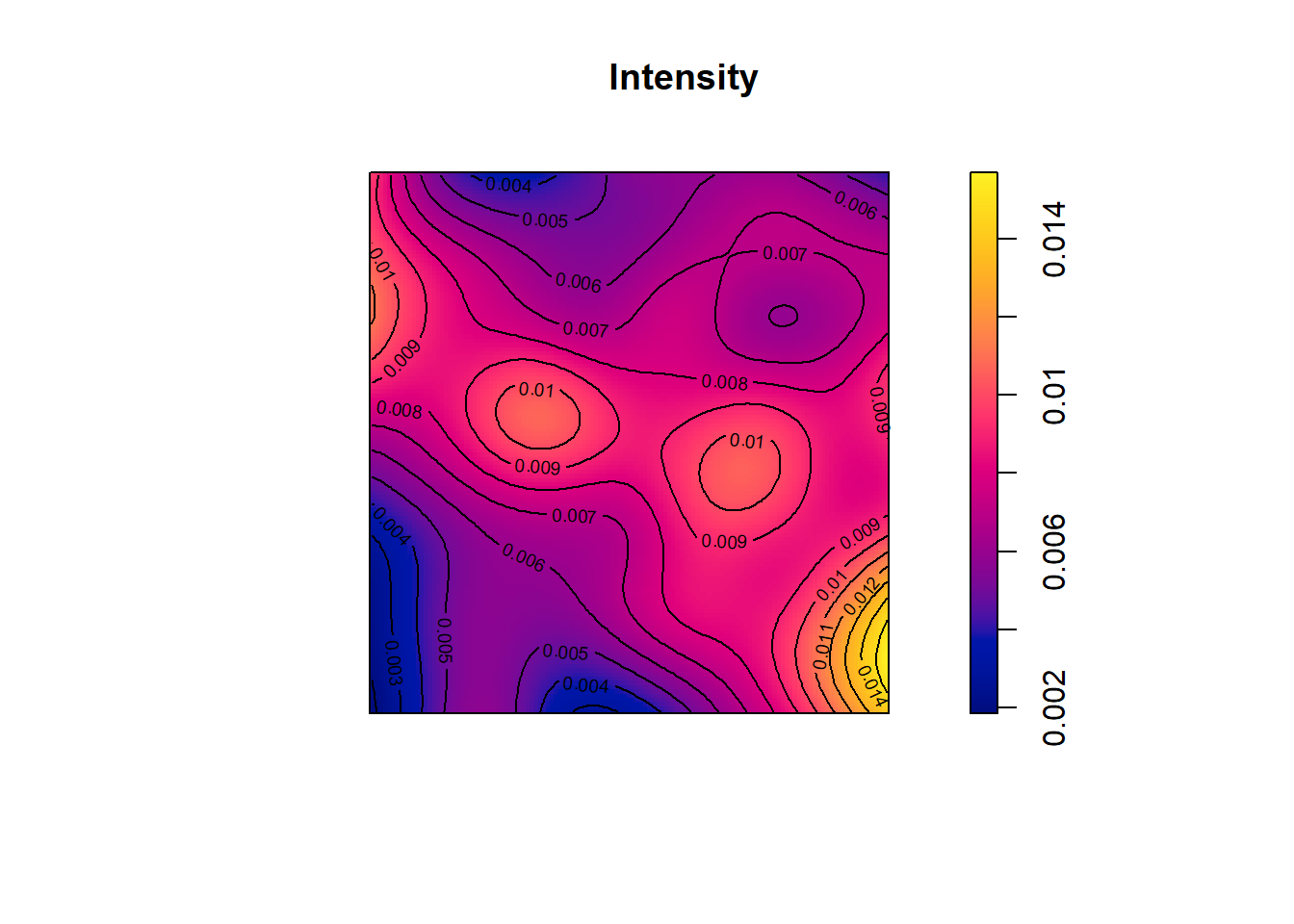
FIGURE 17.1: Locations (top) and intensity (bottom) of 71 trees in a Swedish forest plot.
17.1 Examples
The spatstat package contains a number of examples of spatial point patterns. Here, we describe some of the data included in spatstat, and this document provides an overview of all the data included in the package.
Japanese pines
The japanesepines data from spatstat represents locations of 65 saplings of Japanese pine in a 5.7 \(\times\) 5.7 square meter sampling region in a natural stand (Figure 17.2).
An interesting question when analyzing this data could be whether the spacing between saplings is greater than would be expected for a random pattern (which could indicate competition for resources).
Planar point pattern: 65 points
window: rectangle = [0, 1] x [0, 1] units (one unit =
5.7 metres)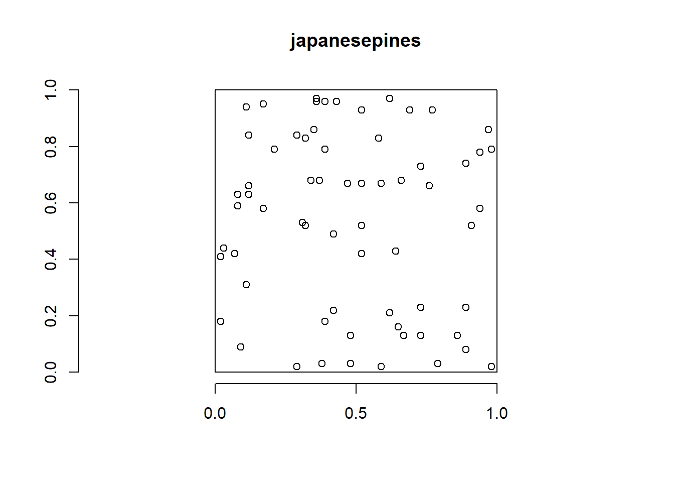
FIGURE 17.2: Locations of 65 saplings of Japanese pine in a natural stand.
Trees in a forest
Spatial point patterns can also have an associated value, and these are called marked point patterns.
An example of marked point pattern is given by the longleaf data from spatstat which contains locations of 584 trees in a forest of longleaf pine trees in Georgia, USA,
along with their diameter at breast height (dbh), a convenient surrogate measure of size and age (Figure 17.3).
Here, it would be interesting to understand the spatial variation in the density and age of trees.
longleafMarked planar point pattern: 584 points
marks are numeric, of storage type 'double'
window: rectangle = [0, 200] x [0, 200] metres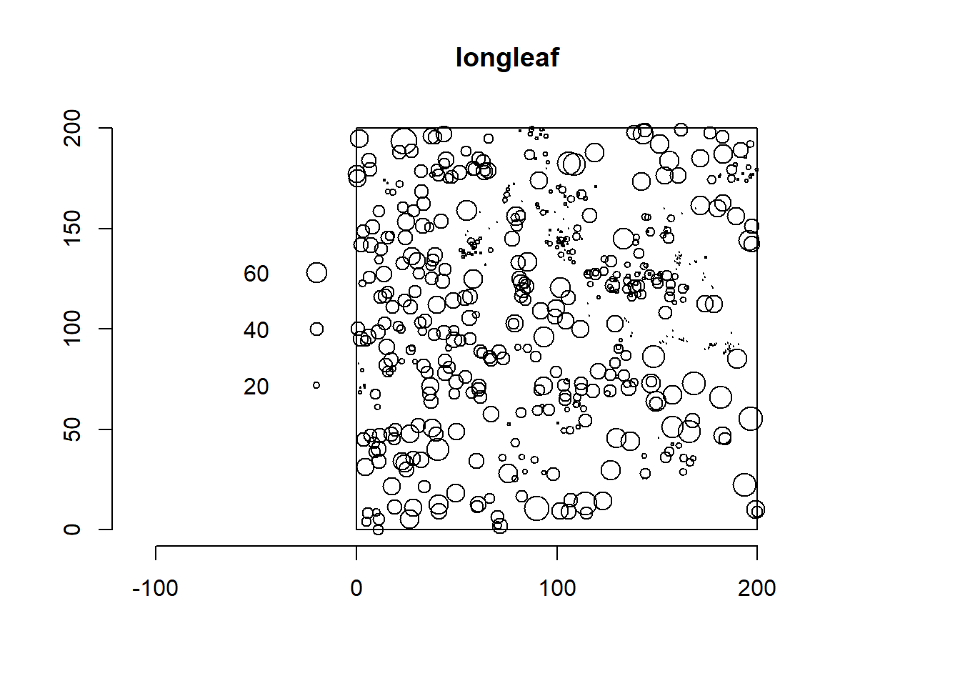
FIGURE 17.3: Locations and diameters of 584 trees in a forest of longleaf pine trees in Georgia, USA.
Castilla-La Mancha forest fires
The clmfires data contains the locations and information of forest fires in the Castilla-La Mancha region of Spain between 1998 and 2007.
Figure ?? shows the fire locations and four marks with information about each fire, namely, the cause of fire (cause),
the total area burned in hectares (burnt.area),
the date of fire (date), and the
number of days elapsed since 1 January 1998 (julian.date).
The main question when analyzing this data could be to understand the spatio-temporal variability of forest fires and potential risk factors.
clmfiresMarked planar point pattern: 8488 points
Mark variables: cause, burnt.area, date, julian.date
window: polygonal boundary
enclosing rectangle: [4.1, 391.4] x [18.6, 385.2]
kilometres
plot(clmfires)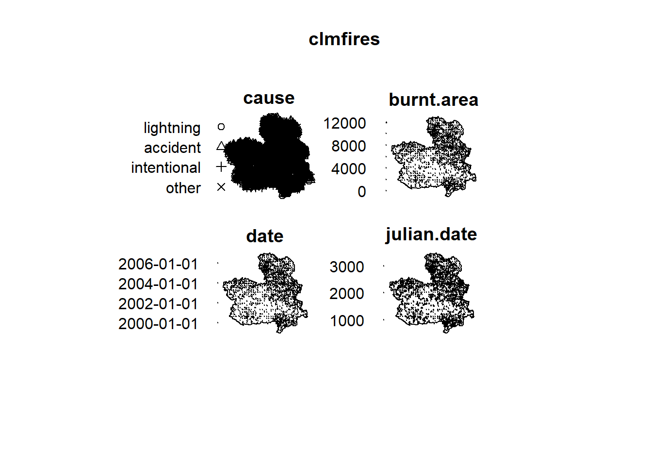
FIGURE 17.4: Locations and information of forest fires in Castilla-La Mancha, Spain.
Hamster tumor data
The hamster data provides the centers of the nuclei of certain cells in a section of tissue from a laboratory-induced lymphoma in the kidney of a hamster (Figure 17.5).
The nuclei are classified as either “pyknotic” (corresponding to dying cells) or “dividing” (corresponding to cells in the act of dividing). The background void is occupied by unrecorded, interphase cells in relatively large numbers.
Using this data, we could investigate how different types of cells interact, and what is the relationship between the degree of cells interaction and cancer stage and survival.
hamsterMarked planar point pattern: 303 points
Multitype, with levels = dividing, pyknotic
window: rectangle = [0, 1] x [0, 1] units (one unit =
250 microns)
plot(hamster)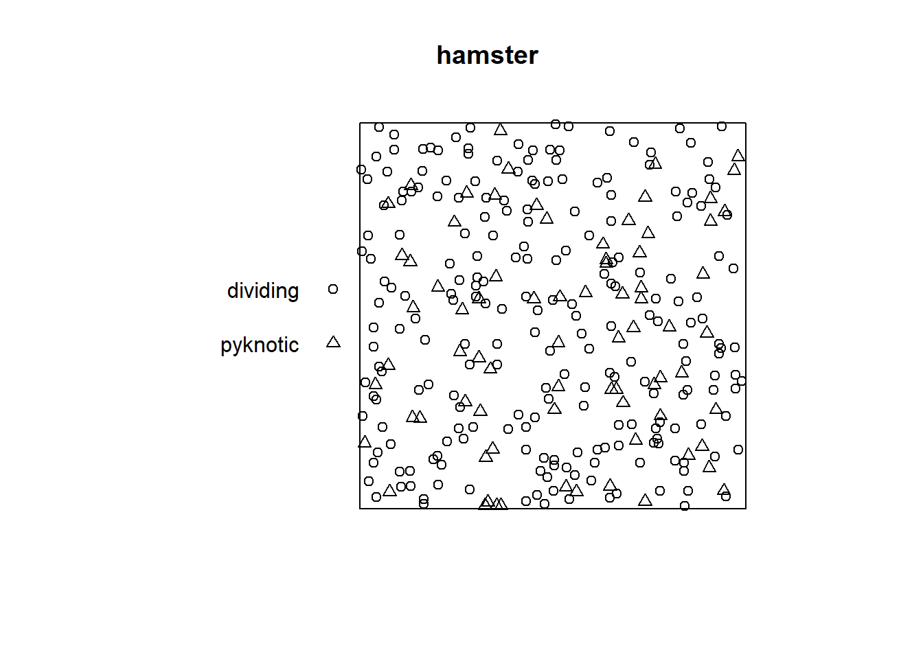
FIGURE 17.5: Cells in a tissue from a lymphoma in the kidney of a hamster.
Chorley-Ribble data
The chorley data gives the addresses of 58 larynx cancer cases and 978 lung cancer cases, recorded in the Chorley and South Ribble Health Authority of Lancashire, England, between 1974 and 1983.
Figure 17.6 shows the locations of the case addresses, as well as the location of a disused industrial incinerator.
After allowing for spatial variation in the density of the susceptible population, we could assess the evidence for an increase in the incidence of larynx cancer near the incinerator. Here, the lung cancer cases could serve as a surrogate for the spatially varying population density.
chorleyMarked planar point pattern: 1036 points
Multitype, with levels = larynx, lung
window: polygonal boundary
enclosing rectangle: [343.4, 366.4] x [410.4, 431.8]
km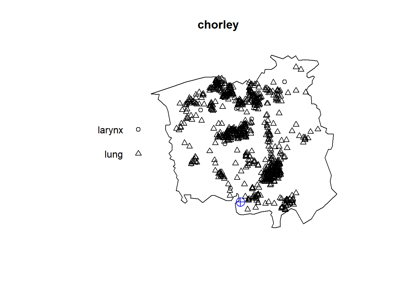
FIGURE 17.6: Locations of larynx and lung cancer cases, and the location of a disused industrial incinerator in a region of Lancashire, England.