23 Point process modeling

23.1 Log-Gaussian Cox processes

Log-Gaussian Cox processes (LGCPs) are typically used to model phenomena that are environmentally driven (Diggle et al. 2013). A LGCP is a Poisson process with a varying intensity, which is itself a stochastic process of the form

\[\Lambda(\boldsymbol{s}) = exp(Z(\boldsymbol{s})),\] where \(Z = \{Z(\boldsymbol{s}) : \boldsymbol{s} \in \mathbb{R^2}\}\) is a Gaussian process. Then, conditional on \(\Lambda(\cdot)\), the point process is an inhomogeneous Poisson process with intensity \(\Lambda(\cdot)\). This implies that the number of events in any region \(A\) is Poisson distributed with mean \(\int_A \Lambda(\boldsymbol{s})d\boldsymbol{s}\), and the locations of events are an independent random sample from the distribution on \(A\) with probability density proportional to \(\Lambda(\cdot)\). A LGCP model can also include spatial explanatory variables providing a flexible approach for describing and predicting a wide range of spatial phenomena.

In this chapter, we assume that we have observed a spatial point pattern of event locations \(\{\boldsymbol{x}_i: i = 1, \ldots, n\}\) that has been generated as a realization of a LGCP, and we show how to fit a LGCP model to the data using the INLA and SPDE approaches. Chapter 15 introduced the SPDE approach and described its implementation in the context of model-based geostatistics using an example of air pollution prediction. Here, we describe how to use SPDE to fit a LGCP model to a point pattern of plant species to estimate the intensity of the process.

23.2 Fitting a LGCP

Grid approach

A common method for inference in LGCP models is to approximate the latent Gaussian field by means of a gridding approach (Illian et al. 2012). In this approach, the study region is first discretized into a regular grid of \(n_1 \times n_2 = N\) cells, \(\{s_{ij}\}\), \(i=1,\ldots,n_1\), \(j=1,\ldots,n_2\). In the LGCP, the mean number of events in cell \(s_{ij}\) is given by the integral of the intensity over the cell, \(\Lambda_{ij} = \int_{s_{ij}} exp(\eta(s)) ds\), and this integral can be approximated by \(\Lambda_{ij} \approx |s_{ij}| exp(\eta_{ij})\), where \(|s_{ij}|\) is the area of the cell \(s_{ij}\). Then, conditional on the latent field \(\eta_{ij}\), the observed number of locations in grid cell \(s_{ij}\), \(y_{ij}\), are independent and Poisson distributed as follows,

\[y_{ij}| \eta_{ij} \sim Poisson(|s_{ij}| exp(\eta_{ij})).\]

Then, the LGCP model can be expressed within the generalized linear mixed model framework. For example, the log-intensity of the Poisson process can be modeled using covariates and random effects as follows:

\[\eta_{ij} = c(s_{ij}) \beta + f_s(s_{ij}) + f_u(s_{ij}).\]

Here, \(\boldsymbol{\beta} = (\beta_0, \beta_1, \ldots, \beta_p)'\) is the coefficient vector of \(\boldsymbol{c}(s_{ij}) = (1, c_1(s_{ij}), \ldots, c_p(s_{ij}))\), the vector of the intercept and covariates values at \(s_{ij}\). \(f_s()\) is a spatially structured random effect reflecting unexplained variability specified as a second-order two-dimensional conditional autoregressive model on a regular lattice. \(f_u()\) is an unstructured random effect reflecting independent variability in the cells. Moraga (2021b) provides an example on how to implement the grid approach to fit a LGCP with INLA using a species distribution modeling study in Costa Rica.

Going off the grid

While the previous approach is a common method for inference in LGCP models, the results obtained depend on the construction of a fine regular grid that cannot be locally refined. An alternative computationally efficient method to perform computational inference on LGCP is presented in Simpson et al. (2016). This method, rather than defining a Gaussian random field over a fine regular grid, proposes a finite-dimensional continuously specified random field of the form

\[Z(\boldsymbol{s}) = \sum_{i=1}^n z_i \phi_i(\boldsymbol{s}),\] where \(\boldsymbol{z} = (z_1, \ldots, z_n)'\) is a multivariate Gaussian random vector and \(\{ \phi_i(\boldsymbol{s})\}_{i=1}^n\) is a set of linearly independent deterministic basis functions. Unlike the lattice approach, this method models observations considering its exact location instead of binning them into cells. Thus, the implementation of this method does not need the specification of a regular grid but a triangulated mesh to approximate the Gaussian random field using the SPDE approach. Below, we give an example of species distribution modeling where we fit a LGCP using this method and INLA and SPDE for fast approximate inference. This approach is also explained in Krainski et al. (2019).

23.3 Species distribution modeling

Species distribution models allow us to understand spatial patterns, and assess the influence of factors on species occurrence. These models are crucial for the development of appropriate strategies that help protect species and the environments where they live. Here, we show how to formulate and fit a LGCP model for Solanum plant species in Bolivia using a continuously Gaussian random field with INLA and SPDE. The model allows us to estimate the intensity of the process that generates the locations.

23.3.1 Observed Solanum plant species in Bolivia

In this example, we estimate the intensity of Solanum plant species in Bolivia from January 2015 to December 2022 which are obtained from the Global Biodiversity Information Facility (GBIF) database with the spocc package. We retrieve the data using the occ() function specifying the plant species scientific name, data source, dates, and country code. We also specify has_coords = TRUE to just return occurrences that have coordinates, and limit = 1000 to specify the limit of the number of records.

library("sf")
library("spocc")

df <- occ(query = "solanum", from = "gbif",
          date = c("2015-01-01", "2022-12-31"),
          gbifopts = list(country = "BO"),
          has_coords = TRUE, limit = 1000)
d <- occ2df(df)

We use the st_as_sf() function to create a sf object called d that contains the nrow(d) = 244 locations retrieved. We set the coordinate reference system (CRS) to EPSG code 4326 since the coordinates of the locations are given by longitude and latitude values.

d <- st_as_sf(d[, 2:3], coords = c("longitude", "latitude"))
st_crs(d) <- "EPSG:4326"

In order to work with kilometers instead of degrees, we project the data to UTM 19S corresponding to the EPSG code 5356 with kilometers as units. To do that, we obtain st_crs("EPSG:5356")$proj4string and change +units=m by +units=km.

st_crs("EPSG:5356")$proj4string
projUTM <- "+proj=utm +zone=19 +south +ellps=GRS80
+towgs84=0,0,0,0,0,0,0 +units=km +no_defs"
d <- st_transform(d, crs = projUTM)

We also obtain the map of Bolivia with the rnaturalearth package, and we project it to UTM 19S with kilometers as units.

library(rnaturalearth)
map <- ne_countries(type = "countries", country = "Bolivia",
                    scale = "medium", returnclass = "sf")
map <- st_transform(map, crs = projUTM)

Figure 23.1 shows a map with the retrieved locations of Solanum plant species in Bolivia.

library("ggplot2")
ggplot() + geom_sf(data = map) +
  geom_sf(data = d) + coord_sf(datum = projUTM)

Finally, we create data frame coo with the event locations.

coo <- st_coordinates(d)

23.3.2 Prediction data

Now, we construct a matrix with the locations coop where we want to predict the point process intensity. To do that, we first create a raster covering the map with the rast() function of terra. Then, we retrieve the coordinates of the cells with the xyFromCell() function of terra.

library(sf)
library(terra)

# raster grid covering map
grid <- terra::rast(map, nrows = 100, ncols = 100)
# coordinates of all cells
xy <- terra::xyFromCell(grid, 1:ncell(grid))

We create a sf object called dp with the prediction locations with st_as_sf(), and use st_filter() to keep the prediction locations that lie within the map. We also retrieve the indices of the points within the map by using st_intersects() setting sparse = FALSE.

# transform points to a sf object
dp <- st_as_sf(as.data.frame(xy), coords = c("x", "y"),
               crs = st_crs(map))

# indices points within the map
indicespointswithin <- which(st_intersects(dp, map,
                                           sparse = FALSE))

# points within the map
dp <- st_filter(dp, map)

Figure 23.1 depicts the prediction locations in the study region.

ggplot() + geom_sf(data = map) +
  geom_sf(data = dp) + coord_sf(datum = projUTM)

We create the matrix coop with the prediction locations.

coop <- st_coordinates(dp)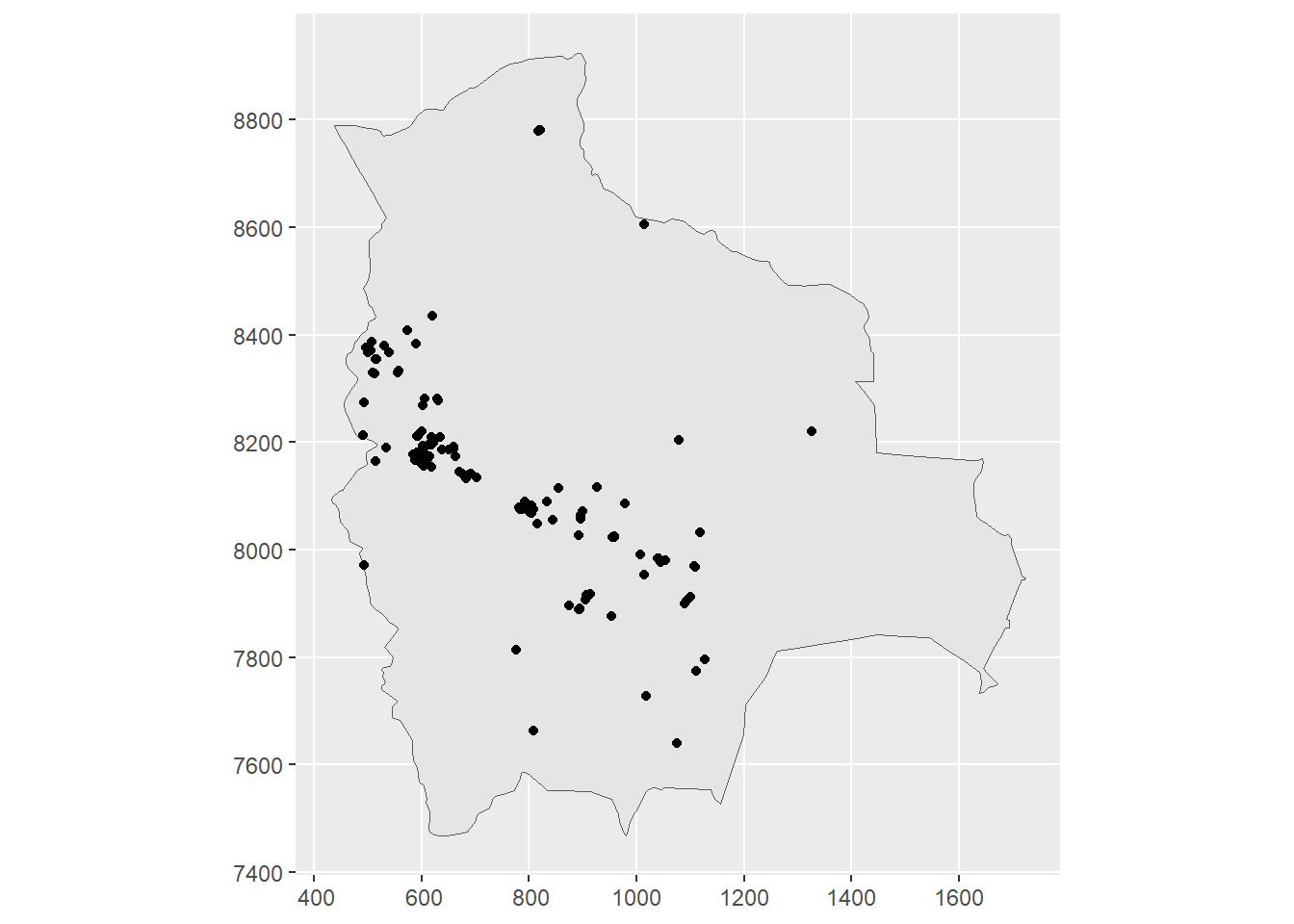

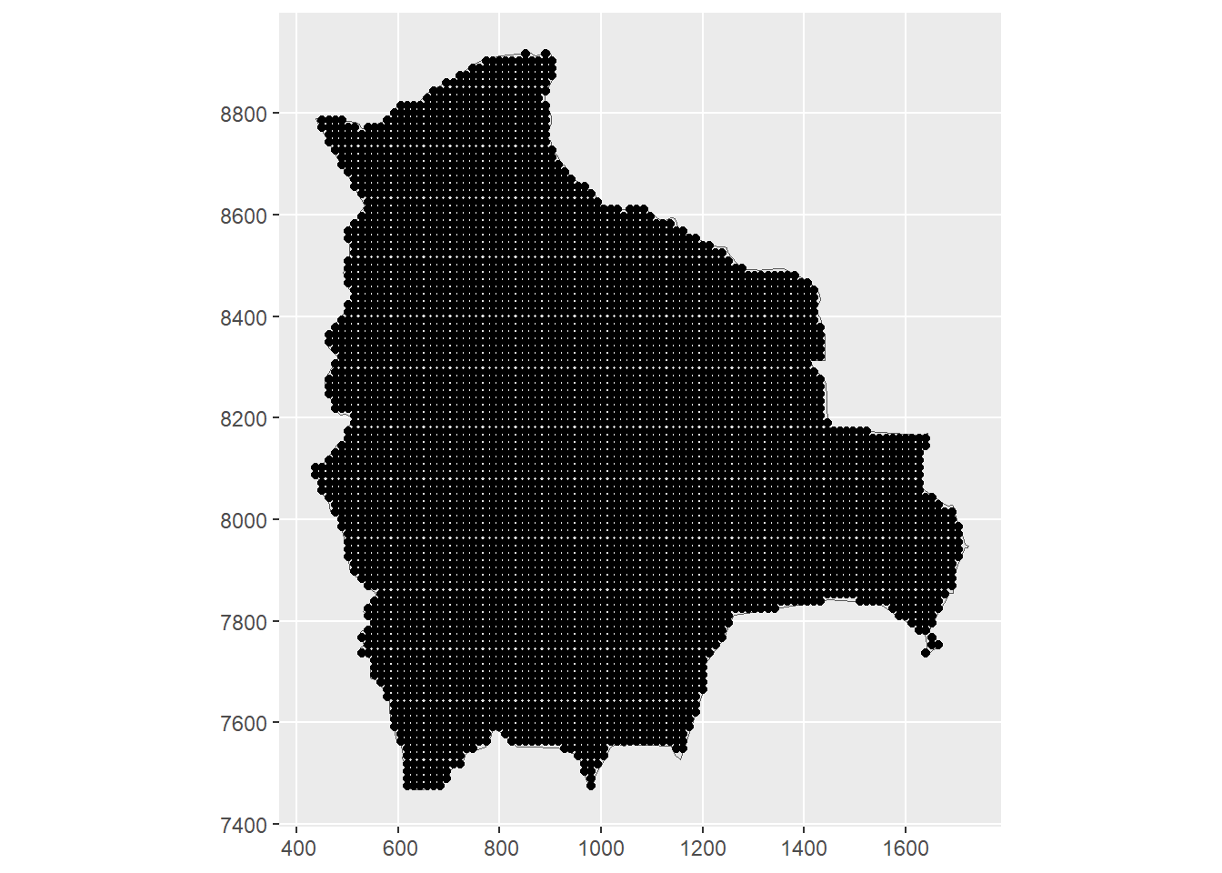
FIGURE 23.1: Left: Locations of Solanum plant species in Bolivia from January 2015 to December 2022 obtained from GBIF. Right: Prediction locations in Bolivia.

23.3.3 Model

We use a LGCP to model the point pattern of plant species. Thus, we assume that the process that originates plant species locations is a Poisson process with a varying intensity expressed as

\[\log(\Lambda(\boldsymbol{s})) = \beta_0 + Z(\boldsymbol{s}),\]

where \(\beta_0\) is the intercept, and \(Z(\cdot)\) is a zero-mean Gaussian spatial process with Matérn covariance function.

23.3.4 Mesh construction

To fit the model using INLA and SPDE, we first construct a mesh. In the analysis of point patterns, we do not usually employ the locations as mesh vertices. We construct a mesh that covers the study region using the inla.mesh.2d() function setting loc.domain equal to a matrix with the point locations of the boundary of the region. Other arguments are as follows. max.edge denotes the maximum allowed triangle edge lengths in the inner region and the extension. offset specifies the size of the inner and outer extensions around the data locations. cutoff is the minimum allowed distance between points that we use to avoid building many small triangles around clustered locations. Figure 23.2 shows the mesh created.

library(INLA)

summary(dist(coo)) # summary of distances between event locations

   Min. 1st Qu.  Median    Mean 3rd Qu.    Max. 
    0.0    65.2   196.8   238.8   382.9  1171.0 

loc.d <- cbind(st_coordinates(map)[, 1], st_coordinates(map)[, 2])

mesh <- inla.mesh.2d(loc.domain = loc.d, max.edge = c(50, 100),
                     offset = c(50, 100), cutoff = 1)

plot(mesh)
points(coo, col = "red")
axis(1)
axis(2)

We also create variables nv with the number of mesh vertices, and the variable n with the number of events of the point pattern. Later, we will use these variables to construct the data stacks.

(nv <- mesh$n)

[1] 1975

(n <- nrow(coo))

[1] 244

We use the inla.spde2.matern() function to build the SPDE model on the mesh.

spde <- inla.spde2.matern(mesh = mesh, alpha = 2, constr = TRUE)

23.3.5 Observed and expected number of events

Here, we create the vectors with the observed and expected number of events. First, we create the dual mesh that consists of a set of polygons around each vertex of the original mesh (Figure 23.2). We can create the dual mesh using the book.mesh.dual() function that is provided in Krainski et al. (2019) and is also written at the end of this chapter.

dmesh <- book.mesh.dual(mesh)
plot(dmesh)
axis(1)
axis(2)

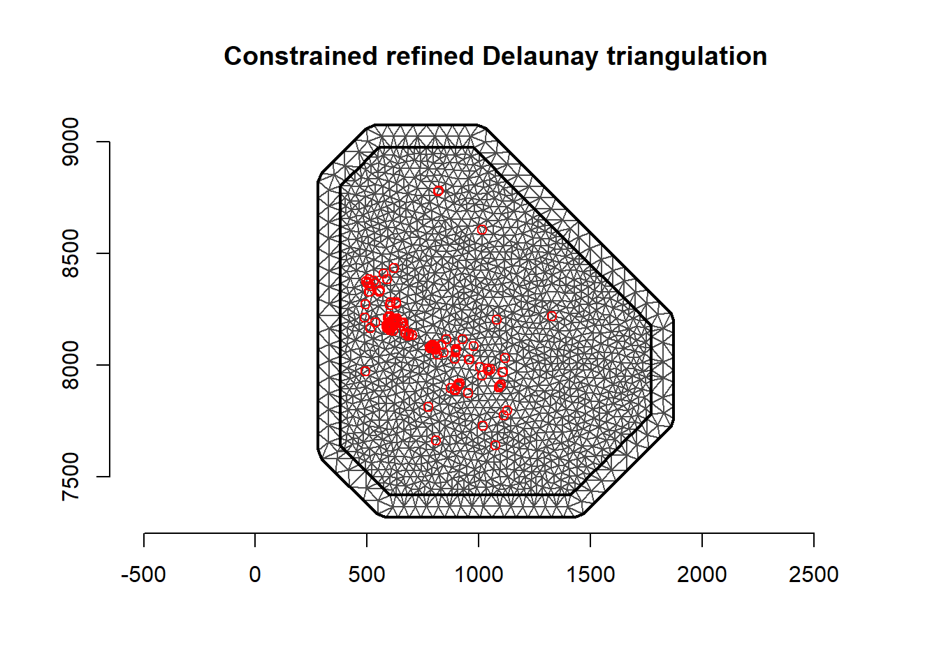
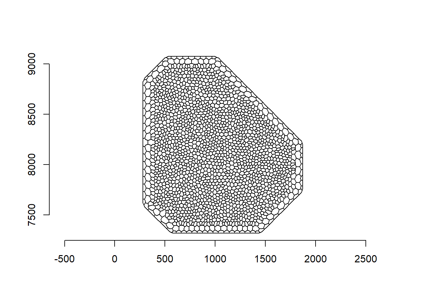
FIGURE 23.2: Mesh (top) and dual mesh (bottom) used in the SPDE approach. Event locations are depicted as red points.

To fit the LGCP, the mesh vertices are considered as integration points. The expected values corresponding to the mesh vertices are proportional to the areas around the mesh vertices, that is, the areas of the polygons of the dual mesh. We calculate a vector of weights called w with the areas of the intersection between each polygon of the dual mesh and the study region using the following code.

# Domain polygon is converted into a SpatialPolygons
domain.polys <- Polygons(list(Polygon(loc.d)), '0')
domainSP <- SpatialPolygons(list(domain.polys))

# Because the mesh is larger than the study area, we need to
# compute the intersection between each polygon
# in the dual mesh and the study area
library(rgeos)

w <- sapply(1:length(dmesh), function(i) {
  if (gIntersects(dmesh[i, ], domainSP))
    return(gArea(gIntersection(dmesh[i, ], domainSP)))
  else return(0)
})

Note that the sum of the weights w is equal to the area of the study region Bolivia.

sum(w) # sum weights

[1] 1093862

st_area(map) # area of the study region

1093862 [km^2]

Figure 23.3 shows the mesh together with the integration points with positive weight in black and with zero weight in red. We observe all points with zero weight are outside the study region.

plot(mesh)
points(mesh$loc[which(w > 0), 1:2], col = "black", pch = 20)
points(mesh$loc[which(w == 0), 1:2], col = "red", pch = 20)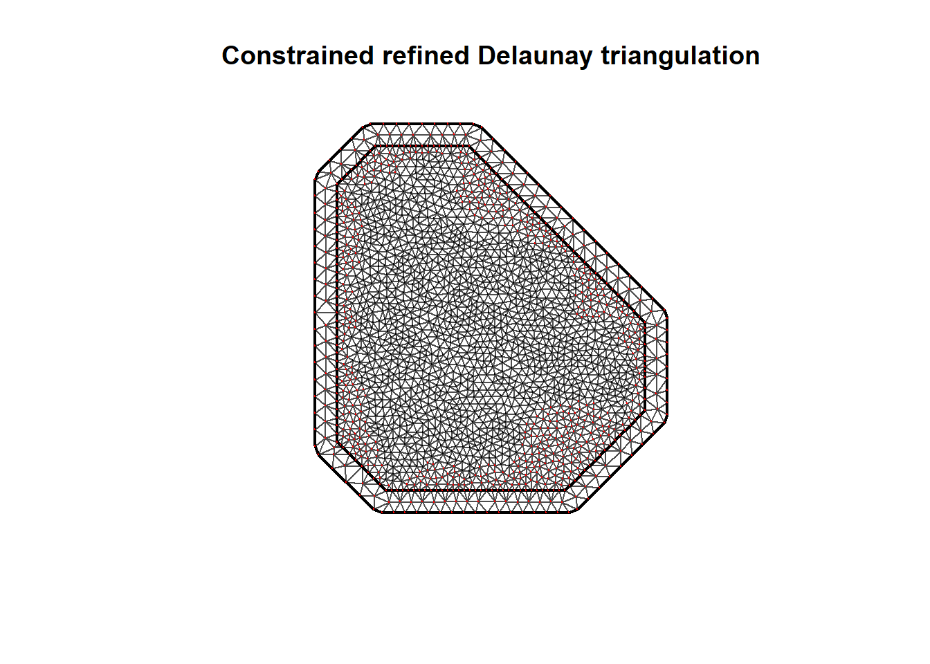

FIGURE 23.3: Mesh together with the points with positive weight in black and with zero weight in red.

Then, we create vectors of the augmented datasets with the observed and the expected values. The observed values will be specified in the model formula as response. The expected values will be specified in the model formula as the component E of the mean for the Poisson likelihood defined as \(E_i exp(\eta_i)\), where \(\eta_i\) is the linear predictor.

Vector y.pp contains the response variable. The first nv elements are 0s corresponding to the mesh vertices. The last n elements are 1s corresponding to the observed events.

Vector e.pp contains the expected values. The first nv elements are the weights w representing the intersection between the areas around each of the mesh vertices and the study region. The following n elements are 0s corresponding to the point events.

y.pp <- rep(0:1, c(nv, n))
e.pp <- c(w, rep(0, n))

head(cbind(y.pp, e.pp))

     y.pp e.pp
[1,]    0    0
[2,]    0    0
[3,]    0    0
[4,]    0    0
[5,]    0    0
[6,]    0    0

tail(cbind(y.pp, e.pp))

        y.pp e.pp
[2214,]    1    0
[2215,]    1    0
[2216,]    1    0
[2217,]    1    0
[2218,]    1    0
[2219,]    1    0

23.3.6 Projection matrix

We construct the projection matrix A.pp to project the Gaussian random field from the observations to the triangulation vertices. This matrix is constructed using the projection matrix for the mesh vertices that is a diagonal matrix (A.int), and the projection matrix for the event locations (A.y).

# Projection matrix for the integration points (mesh vertices)
A.int <- Diagonal(nv, rep(1, nv))
# Projection matrix for observed points (event locations)
A.y <- inla.spde.make.A(mesh = mesh, loc = coo)
# Projection matrix for mesh vertices and event locations
A.pp <- rbind(A.int, A.y)

We also create the projection matrix Ap.pp for the prediction locations.

Ap.pp <- inla.spde.make.A(mesh = mesh, loc = coop)

23.3.7 Stack with data for estimation and prediction

Now we use the inla.stack() function to construct stacks for estimation and prediction that organize the data, effects, and projection matrices. In the arguments of inla.stack(), data is a list with the observed (y) and expected (e) values. Argument A contains the projection matrices, and argument effects is a list with the fixed and random effects. Then, the estimation and prediction stacks are combined in a full stack.

# stack for estimation
stk.e.pp <- inla.stack(tag = "est.pp",
data = list(y = y.pp, e = e.pp), 
A = list(1, A.pp),
effects = list(list(b0 = rep(1, nv + n)), list(s = 1:nv)))

# stack for prediction stk.p
stk.p.pp <- inla.stack(tag = "pred.pp",
data = list(y = rep(NA, nrow(coop)), e = rep(0, nrow(coop))),
A = list(1, Ap.pp),
effects = list(data.frame(b0 = rep(1, nrow(coop))),
               list(s = 1:nv)))

# stk.full has stk.e and stk.p
stk.full.pp <- inla.stack(stk.e.pp, stk.p.pp)

23.3.8 Model formula and inla() call

The formula is specified by including the response in the left-hand side and the random effects in the right-hand side.

formula <- y ~ 0 + b0 + f(s, model = spde)

We fit the model by calling inla(). In the function, we specify link = 1 to compute the fitted values that are given in res$summary.fitted.values and res$marginals.fitted.values with the same link function as the family specified in the model.

res <- inla(formula,  family = 'poisson',
data = inla.stack.data(stk.full.pp),
control.predictor = list(compute = TRUE, link = 1,
                         A = inla.stack.A(stk.full.pp)),
E = inla.stack.data(stk.full.pp)$e)

23.3.9 Results

A summary of the results can be inspected by typing summary(res). The data frame res$summary.fitted.values contains the fitted values. The indices of the rows corresponding to the predictions can be obtained with inla.stack.index() specifying the tag "pred.pp" of the prediction stack.

index <- inla.stack.index(stk.full.pp, tag = "pred.pp")$data
pred_mean <- res$summary.fitted.values[index, "mean"]
pred_ll <- res$summary.fitted.values[index, "0.025quant"]
pred_ul <- res$summary.fitted.values[index, "0.975quant"]

Then, we add layers to the grid raster with the posterior mean, and 2.5 and 97.5 percentiles values in the cells that are within the map.

grid$mean <- NA
grid$ll <- NA
grid$ul <- NA

grid$mean[indicespointswithin] <- pred_mean
grid$ll[indicespointswithin] <- pred_ll
grid$ul[indicespointswithin] <- pred_ul

Finally, we create maps of the posterior mean and the lower and upper limits of 95% credible intervals of the intensity of the point process of species in Bolivia (Figure 23.4). To do that, we use the levelplot() function of the rasterVis package specifying names.attr with the name of each panel and layout with the number of columns and rows.

library(rasterVis)
levelplot(raster::brick(grid), layout = c(3, 1),
names.attr = c("Mean", "2.5 percentile", "97.5 percentile"))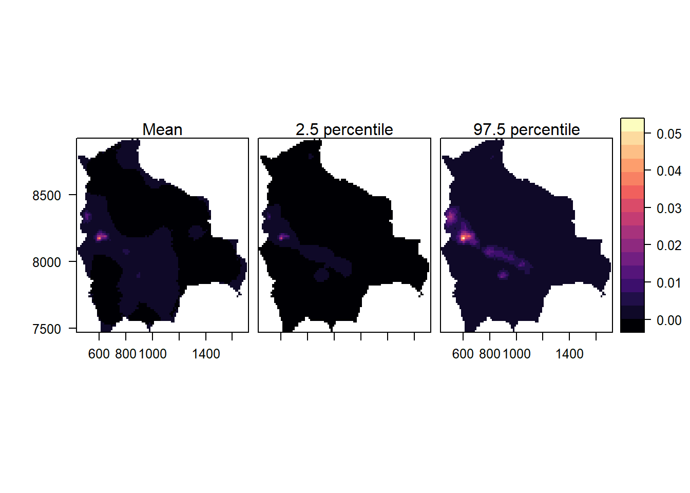

FIGURE 23.4: Maps with the posterior mean of the intensity of the point process of species in Bolivia (left), and lower (center) and upper (right) limits of 95% credible intervals.

Overall, we observe a low intensity of species, with higher intensity in the central west part of Bolivia. Note that we have modeled species occurrence data retrieved from GBIF by assuming the observed spatial point pattern is a realization of the underlying process that generates the species locations. In real applications, it is important to understand how data was collected, and assess potential data biases such as overrepresentation of certain areas that can invalidate the results. Moreover, it is important to incorporate expert knowledge, to create models that include relevant covariates and random effects to account for various types of variability, enabling a more comprehensive understanding of the variable under investigation.

23.3.10 Function to create the dual mesh

The following code corresponds to the book.mesh.dual() function to create the dual mesh.

book.mesh.dual <- function(mesh) {
    if (mesh$manifold=='R2') {
        ce <- t(sapply(1:nrow(mesh$graph$tv), function(i)
            colMeans(mesh$loc[mesh$graph$tv[i, ], 1:2])))
        library(parallel)
        pls <- mclapply(1:mesh$n, function(i) {
            p <- unique(Reduce('rbind', lapply(1:3, function(k) {
            j <- which(mesh$graph$tv[,k]==i)
            if (length(j)>0) 
            return(rbind(ce[j, , drop=FALSE],
            cbind(mesh$loc[mesh$graph$tv[j, k], 1] +
            mesh$loc[mesh$graph$tv[j, c(2:3,1)[k]], 1], 
            mesh$loc[mesh$graph$tv[j, k], 2] +
            mesh$loc[mesh$graph$tv[j, c(2:3,1)[k]], 2])/2))
            else return(ce[j, , drop=FALSE])
            })))
            j1 <- which(mesh$segm$bnd$idx[,1]==i)
            j2 <- which(mesh$segm$bnd$idx[,2]==i)
            if ((length(j1)>0) | (length(j2)>0)) {
            p <- unique(rbind(mesh$loc[i, 1:2], p,
            mesh$loc[mesh$segm$bnd$idx[j1, 1], 1:2]/2 +
            mesh$loc[mesh$segm$bnd$idx[j1, 2], 1:2]/2, 
            mesh$loc[mesh$segm$bnd$idx[j2, 1], 1:2]/2 +
            mesh$loc[mesh$segm$bnd$idx[j2, 2], 1:2]/2))
            yy <- p[,2]-mean(p[,2])/2-mesh$loc[i, 2]/2
            xx <- p[,1]-mean(p[,1])/2-mesh$loc[i, 1]/2
            }
            else {
            yy <- p[,2]-mesh$loc[i, 2]
            xx <- p[,1]-mesh$loc[i, 1]
            }
            Polygon(p[order(atan2(yy,xx)), ])
        })
        return(SpatialPolygons(lapply(1:mesh$n, function(i)
            Polygons(list(pls[[i]]), i))))
    }
    else stop("It only works for R2!")
}