11 Categorical variables
11.1 Categorical variables
\[Y_i = \beta_0 + \beta_1 X_{i1} + \beta_2 X_{i2} + \ldots + \beta_p X_{ip} + \epsilon_i,\ \ \epsilon_i \sim^{iid} N(0, \sigma^2),\ \ i = 1,\ldots,n\]
Sometimes we want to include a categorical explanatory variable in the model.
Example: what is the relationship between income and education level allowing for gender (male or female)?
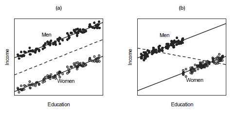
- The figure shows examples on the relationship between education and income among women and men.
- In both cases, the within-gender regressions of income on education are parallel. Parallel regressions imply additive effects of education and gender on income.
- In (a), gender and education are unrelated to each other. If we ignore gender and regress income on education alone, we obtain the same slope as in the separate within-gender regressions. Ignoring gender inflates the size of the errors, however.
- In (b) gender and education are related (women have higher average education than men). Therefore, if we regress income on education alone, we obtain a biased assessment of the effect of education on income. The overall regression of income on education has a negative slope even though the within-gender regressions have positive slopes.
11.2 Categorical variables with 2 categories
We want to understand the relationship between income (\(Y\), continuous response variable) and gender (categorical explanatory variable) and education (\(X\), continuous explanatory variable).
To include a categorical explanatory variable with \(M\) categories in the model, we choose a reference category and include \(M-1\) indicator variables that represent the other categories of the categorical explanatory variable. Indicator variables are also called dummy variables and take values 0 or 1.
Gender is a categorical explanatory variable with two categories: men and women. We choose women as the reference category and create 2-1 dummy variables:
- \(D\) = 1 if Men and 0 otherwise (Women)
| Gender | \(D\) |
| Men | 1 |
| Women | 0 |
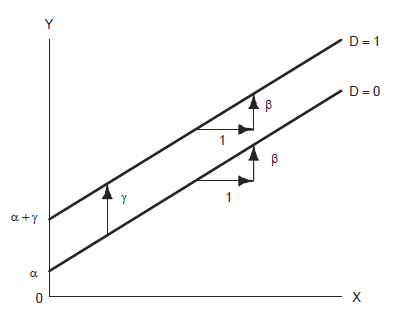
We assume an additive model (the partial effect of each explanatory variable is the same regardless of the specific value at which the other explanatory variable is held constant). One way of formulating the common slope model is
\[Y_i = \alpha + \beta X_i + \gamma D_i + \epsilon_i\]
For women, \(Y_i = \alpha + \beta X_i + \gamma (0) + \epsilon_i = \alpha + \beta X_i + \epsilon_i\)
For men, \(Y_i = \alpha + \beta X_i + \gamma (1) + \epsilon_i = (\alpha + \gamma) + \beta X_i + \epsilon_i\)
\(\gamma\) is the difference in the mean value of income between men and the reference category women
11.3 Categorical variables with more than 2 categories
We want to understand the relationship between prestige (\(Y\)) and categorical variable occupation and continuous variables income (\(X_1\)) and education (\(X_2\)).
Occupations are classified into three categories: professional and managerial, white-collar and blue-collar. We choose Blue Collar as the reference category and create 3-1=2 dummy variables.
\(D_1\) = 1 if Professional & Managerial and 0 otherwise (White Collar and Blue Collar)
\(D_2\) = 1 if White Collar and 0 otherwise (Professional & Managerial and Blue Collar)
| Category | \(D_1\) | \(D_2\) |
| Professional & Managerial | 1 | 0 |
| White Collar | 0 | 1 |
| Blue Collar | 0 | 0 |
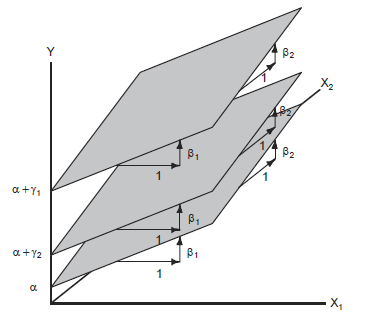
\[Y_i = \alpha + \beta_1 X_{i1} + \beta_2 X_{i2} + \gamma_1 D_{i1} + \gamma_2 D_{i2} + \epsilon_i\]
Professional: \(Y_i = (\alpha + \gamma_1) + \beta_1 X_{i1} + \beta_2 X_{i2} + \epsilon_i\)
White-collar: \(Y_i = (\alpha + \gamma_2) + \beta_1 X_{i1} + \beta_2 X_{i2} + \epsilon_i\)
Blue-collar: \(Y_i = \alpha + \beta_1 X_{i1} + \beta_2 X_{i2} + \epsilon_i\)
This model describes three parallel regression planes which can differ in their intercepts
\(\alpha\) is the intercept for blue-collar occupations
\(\gamma_1\) represents the constant vertical distance between the parallel regression planes for professional and blue-collar occupations (fixing the values of education and income)
\(\gamma_2\) represents the constant vertical distance between the regression planes for white-collar and blue-collar occupations (fixing the values of education and income)
Blue-collar occupations are coded 0 for both dummy regressors, so Blue-collar serves as a baseline category with which the other occupational categories are compared
\(\gamma_j\) is the difference in the mean value of \(Y\) between category \(j\) and the reference category (holding the rest of covariates constant)
11.4 Including a categorical variable in the model
Including a categorical variable with M categories in the model:
- Choose a category as reference category
- Create M-1 dummy variables
- Include the dummy variables in the model
- The coefficients of the dummy variables indicate the increase or decrease in the mean value of \(Y\) with respect reference category.
For example, consider a categorical variable with categories 1, 2, \(\ldots\), M. We consider the reference category as 1, and create the following dummy variables:
\(D_2\) = 1 if category 2 and 0 otherwise
\(D_3\) = 1 if category 3 and 0 otherwise
…
\(D_M\) = 1 if category 1 and 0 otherwise
\[Y = \alpha + \beta_2 D_2 + \beta_3 D_3 + \ldots + \beta_M D_M + \epsilon\] \(\beta_j\) is the difference in the mean value of \(Y\) between category \(j\) and the reference category (holding the rest of covariates constant).
11.5 Example. Organization’s income
In a large organization, we obtained data on yearly income for the employees. By computing sample means for the income of male employees it appears that this is larger than the mean salary for female employees. There is concern about this, and since you are the organization’s statistical expert, you are asked to check whether there is a significant difference in the income between genders. How would you proceed using linear regression? Write the model and explain the procedure you would follow.
Consider the model for the response variable “income” with independent variables “gender” and “experience”, the latter categorised as “junior”, “intermediate” and “senior”. Write the additive model by considering the main effects of the covariates, and by choosing the baseline categories “male’’ for”gender” and “junior” for “experience”. Then write the expected income of a junior male employee. Finally, write the model for the expected income of a senior female employee.
We fit the model having covariates gender and experience. Then we obtained from R the summary of this fit and noticed that the estimated coefficients for the “intermediate” and “senior” experience levels were positive and significant at the chosen significance level \(\alpha\), and that all the remaining coefficients were non-significant. You have to write a report and explain carefully what this implies. What would you report?
Solution
Gender is a categorical variable. Here, we set baseline gender = male. We have the linear model
\[E(income | gender) = \beta_0 + \beta_1 \times X_{female},\]
with dummy variable \(X_{female} = 1\) for female subjects and 0 otherwise.
\(\beta_0\) is the expected income for a male employee, and \(\beta_0+\beta_1\) the expected income for a female employee. Therefore, \(\beta_1\) represents the difference in income between genders.
To check whether there is a significant difference in the income between genders we would test the hypothesis \(H_0 : \beta_1 = 0\) versus the alternative hypothesis \(H_1 : \beta_1 \neq 0\). We can use a t-test for this task at some significance level \(\alpha\). If we reject \(H_0\) then we conclude that there is a significant difference.
We choose the following baselines: baseline gender = male and baseline experience = junior. The model with main effects only is
\[E(income|gender, experience) = \beta_0 + \beta_1 \times X_{female} + \beta_2 \times X_{intermediate} + \beta_3 \times X_{senior}.\]
We have that \(\beta_0\) is the expected income for a junior male (all introduced dummy variables are zero in this case). \(\beta_0 + \beta_1 + \beta_3\) is the expected income for a senior female.
This means that, marginally with respect to gender (i.e. regardless of the gender), employees with intermediate experience and senior experience are earning on average more than junior employees. Also, marginally with respect to the experience level, there is no difference in income between different genders.
11.6 Example. Breast cancer study
In a German breast cancer case study in Germany from 1984-1989, there were 686 observations including variables tumor size (measured in mm), age, menopausal status (meno), number of positive lymph nodes (nodes), progesterone receptor (pgr) and oestrogen (er).
Are the variables age, menopausal status, number of positive lymph nodes, progesterone receptor and oestrogen useful to explain tumor size?
d <- read.csv("data/GermanBreastCancer.csv")
head(d[, c("size", "age", "meno", "nodes", "pgr", "er")])
size age meno nodes pgr er
1 18 49 premenopausal 2 0 0
2 20 55 postmenopausal 16 0 0
3 40 56 postmenopausal 3 0 0
4 25 45 premenopausal 1 0 4
5 30 65 postmenopausal 5 0 36
6 52 48 premenopausal 11 0 0Response variable is tumour size (size)
Covariates:
- Menopausal status (
meno) is a categorical variable - Age (
age), number of positive lymph nodes (nodes), progesterone receptor (pgr), oestrogen (er) are continuous variables. Number of positive lymph nodes is a count variable (nodes) that can be considered as continuous variable
Create indicator variable
Menopausal status is a categorical variable with two categories: premenopausal and postmenopausal.
We choose one category as reference and create a indicator variable for the other category. For example, we can set postmenopausal as the reference category and create an indicator variable called pre for category premenopausal:
pre = 1if menopausal status is premenopausal
pre = 0if menopausal status is postmenopausal
d$pre <- as.numeric(as.factor(d$meno)) - 1
head(d[, c("meno", "pre")])
meno pre
1 premenopausal 1
2 postmenopausal 0
3 postmenopausal 0
4 premenopausal 1
5 postmenopausal 0
6 premenopausal 1Interpretation of coefficients and p-values
res <- lm(size ~ age + nodes + pgr + er + pre, data = d)
summary(res)
Call:
lm(formula = size ~ age + nodes + pgr + er + pre, data = d)

Residuals:
    Min      1Q  Median      3Q     Max
-39.742  -8.684  -2.391   5.745  84.350

Coefficients:
             Estimate Std. Error t value Pr(>|t|)
(Intercept) 27.429281   4.860937   5.643 2.46e-08 ***
age         -0.040185   0.081692  -0.492    0.623
nodes        0.855936   0.094620   9.046  < 2e-16 ***
pgr          0.001734   0.002792   0.621    0.535
er          -0.006082   0.003870  -1.571    0.117
pre          0.327211   1.642781   0.199    0.842
---
Signif. codes:  0 '***' 0.001 '**' 0.01 '*' 0.05 '.' 0.1 ' ' 1

Residual standard error: 13.51 on 680 degrees of freedom
Multiple R-squared:  0.1138,    Adjusted R-squared:  0.1073
F-statistic: 17.47 on 5 and 680 DF,  p-value: 2.691e-16
\[\widehat{\mbox{size}} = 27.43 -0.0402 \mbox{ age} + 0.8559 \mbox{ nodes} + 0.00173 \mbox{ pgr} - 0.00608 \mbox{ er} + 0.33 \mbox{ pre}\]
If
menopostmenopausal (pre = 0), \(0.33 \times pre = 0.33 \times 0 = 0\) and intercept is \((27.43+0)\)
\(\widehat{\mbox{size}}\) = 27.43 - 0.0402 age + 0.8559 nodes + 0.00173 pgr - 0.00608 erIf
menopremenopausal (pre = 1), \(0.33\times pre = 0.33 \times 1 = 0.33\) and intercept is \((27.43+0.33)\)
\(\widehat{\mbox{size}}\) = 27.76 - 0.0402 age + 0.8559 nodes + 0.00173 pgr - 0.00608 er27.43 is the mean size when
age = nodes = pgr = er = pre = 00.33 is the difference in the mean size between
pre = 1andpre = 0, given that the rest of variables remain constant. p-value=0.842, there is not evidence thatpreaffects the mean size allowing for the other predictorsmean size decreases by 0.0402 for every unit increase in
age, given that the rest of variables remain constant. p-value=0.623, there is not evidence thatageaffects the mean size allowing for the other predictorsmean size increases by 0.8559 for every unit increase in
nodes, given that the rest of variables remain constant. p-value=0.000, there is strong evidence thatnodesaffects the mean size allowing for the other predictorsmean size increases by 0.00173 for every unit increase in
pgr, given that the rest of variables remain constant. p-value=0.535, there is not evidence thatpgraffects the mean size allowing for the other predictorsmean size decreases by 0.00608 for every unit increase in
er, given that the rest of variables remain constant. p-value=0.117, there is not evidence thateraffects the mean size allowing for the other predictors
11.7 Comparison ANOVA and regression
Testing whether there is an association between a continuous dependent variable and a categorical independent variable is equivalent to testing whether there is a significantly difference between the mean of the categories.
ANOVA and regression are statistically equivalent and can test the same hypothesis. However regression analysis is a more flexible approach because it encompasses more data analytic situations (e.g., prediction, continuous independent variables, etc.). Let us see an example:
Data
The data PlantGrowth contain the results from an experiment to compare weight of plants obtained under a control and two different treatment conditions.
d <- PlantGrowth
summary(d)
weight group
Min. :3.590 ctrl:10
1st Qu.:4.550 trt1:10
Median :5.155 trt2:10
Mean :5.073
3rd Qu.:5.530
Max. :6.310 nrow(d)[1] 30levels(d$group)[1] "ctrl" "trt1" "trt2"We use a model with a response variable weight and a single categorical explanatory variable group with 3 categories: ctrl, trt1 and trt2.
We can run this as either an ANOVA or a regression.
ANOVA
\(H_0: \mu_{ctrl} = \mu_{trt1} = \mu_{trt2}\)
\(H_1:\) At least one population mean is different
In ANOVA, the F statistic compares the variation between groups to the variation within groups. \[F = \frac{SSB/(k-1)}{SSW/(n-k)} = \frac{MSB}{MSW} \sim F(k-1, n-k) = F(3-1, 30-3)\]
res <- aov(weight ~ group, data = d)
summary(res)
Df Sum Sq Mean Sq F value Pr(>F)
group 2 3.766 1.8832 4.846 0.0159 *
Residuals 27 10.492 0.3886
---
Signif. codes: 0 '***' 0.001 '**' 0.01 '*' 0.05 '.' 0.1 ' ' 1ANOVA table
| Source | SS | df | MS | F | P |
|---|---|---|---|---|---|
| Between(Group) | SSB | k-1 | MSB=SSB/(k-1) | MSB/MSW | P |
| Within(Error) | SSW | n-k | MSW=SSW/(n-k) | ||
| Total | SST | n-1 |
\[\mbox{SST = SSB + SSW}\]
SS: Sum of Squares (Sum of Squares of the deviations)
- SSB = \(\sum_k n_k(\bar x_k-\bar x)^2\) variation BETWEEN groups.
- SSW = \(\sum_k \sum_i (x_{ik}-\bar x_{k})^2\) variation WITHIN the groups or unexplained random error.
- SST = \(\sum_k \sum_i (x_{ik}-\bar x)^2\) TOTAL variation in the data from the grand mean.
df: Degrees of freedom
- Degrees of freedom of SSB = \(k-1\). Variation of the \(k\) group means about the overall mean
- Degrees of freedom of SSW = \(n-k\). Variation of the \(n\) observations about \(k\) group means
- Degrees of freedom of SST = \(n-1\). Variation of all \(n\) observations about the overall mean
Regression
In a linear regression, we consider ctrl as the reference category and create two dummy variables (0/1):
grouptrt1= 1 if group istrt1and 0 otherwisegrouptrt2= 1 if group istrt2and 0 otherwise
This means that observations in the reference group ctrl have variables trt1 and trt2 equal to 0.
We fit the model \[E[Y] = \beta_0 + \beta_1 \times trt1 + \beta_2 \times trt2\]
- \(\beta_0\) is the mean weight when
trt1andtrt2are 0. That is, \(\beta_0\) is the mean weight for the categoryctrl. - \(\beta_1\) is the mean weight difference between
trt1andctrl. - \(\beta_2\) is the mean weight difference between
trt2andctrl.
Set the reference value of the factor variable group to ctrl
d$group <- relevel(d$group, ref = "ctrl")Run regression
summary(lm(weight ~ group, data = d))
Call:
lm(formula = weight ~ group, data = d)

Residuals:
    Min      1Q  Median      3Q     Max
-1.0710 -0.4180 -0.0060  0.2627  1.3690

Coefficients:
            Estimate Std. Error t value Pr(>|t|)
(Intercept)   5.0320     0.1971  25.527   <2e-16 ***
grouptrt1    -0.3710     0.2788  -1.331   0.1944
grouptrt2     0.4940     0.2788   1.772   0.0877 .
---
Signif. codes:  0 '***' 0.001 '**' 0.01 '*' 0.05 '.' 0.1 ' ' 1

Residual standard error: 0.6234 on 27 degrees of freedom
Multiple R-squared:  0.2641,    Adjusted R-squared:  0.2096
F-statistic: 4.846 on 2 and 27 DF,  p-value: 0.01591
Results
In both ANOVA and regression, \(F\) = 4.846 and p-value = 0.0159. Results are significant.
In ANOVA this indicates at least two means are significantly different.
\(H_0: \mu_{ctrl} = \mu_{trt1} = \mu_{trt2}\)
\(H_1:\) At least one population mean is different
\(F = \frac{SSB/(k-1)}{SSW/(n-k)} = \frac{MSB}{MSW} \sim F(k-1, n-k) = F(3-1, 30-3)\)
In regression, the F test indicates at least one of \(\beta_1\) and \(\beta_2\) are different from 0.
\(H_0\): \(\beta_{1} =\beta_{2} = 0\) (all coefficients are 0)
\(H_1\): at least one of \(\beta_1\), \(\beta_2 \neq 0\) (not all coefficients are 0)
\(F = \frac{\sum_{i=1}^n (\hat Y_i - \bar Y)^2/p}{\sum_{i=1}^n ( Y_i - \hat Y_i)^2/(n-p-1)} = \frac{SSM/df_M}{SSE/df_E} = \frac{MSM}{MSE} \sim F(p, n-p-1)\)
By using the regression model, we obtain the mean of the reference group (as an intercept), and the differences between the reference group mean and all the other means, and also p-values that evaluate those specific comparisons.
- intercept = 5.0320 is the mean of the reference group
ctrl trt1= -0.3710 is the difference in the mean between grouptrt1and the reference groupctrltrt2= 0.4940 is the difference in the mean between grouptrt2and the reference groupctrl.
Regression F test
\(H_0\): \(\beta_{1} =\beta_{2}=...=\beta_{p}\) = 0 (all coefficients are 0)
\(H_1\): at least one of \(\beta_1\), \(\beta_2\), \(\dots\), \(\beta_p \neq\) 0 (not all coefficients are 0)
| Source | Sum of Squares | degrees of freedom | Mean square | F | p-value |
|---|---|---|---|---|---|
| Model | SSM | p | MSM=SSM/p | MSM/MSE | Tail area above F |
| Error | SSE | n-p-1 | MSE=SSE/(n-p-1) | ||
| Total | SST | n-1 |
Under \(H_0\):
\[F = \frac{\sum_{i=1}^n (\hat Y_i - \bar Y)^2/p}{\sum_{i=1}^n ( Y_i - \hat Y_i)^2/(n-p-1)} = \frac{SSM/df_M}{SSE/df_E} = \frac{MSM}{MSE} \sim F(p, n-p-1)\]