d <-read.table("data/patsat.txt", header =TRUE)res <-lm(Satisfaction ~ Age + Severity + Anxiety, data = d)summary(res)
Call:
lm(formula = Satisfaction ~ Age + Severity + Anxiety, data = d)

Residuals:
    Min      1Q  Median      3Q     Max
-16.954  -7.154   1.550   6.599  14.888

Coefficients:
            Estimate Std. Error t value Pr(>|t|)
(Intercept) 162.8759    25.7757   6.319 4.59e-06 ***
Age          -1.2103     0.3015  -4.015  0.00074 ***
Severity     -0.6659     0.8210  -0.811  0.42736
Anxiety      -8.6130    12.2413  -0.704  0.49021
---
Signif. codes:  0 '***' 0.001 '**' 0.01 '*' 0.05 '.' 0.1 ' ' 1

Residual standard error: 10.29 on 19 degrees of freedom
Multiple R-squared:  0.6727,    Adjusted R-squared:  0.621
F-statistic: 13.01 on 3 and 19 DF,  p-value: 7.482e-05
17.2 Checking assumptions linear model
Independence
Random sample
Normality
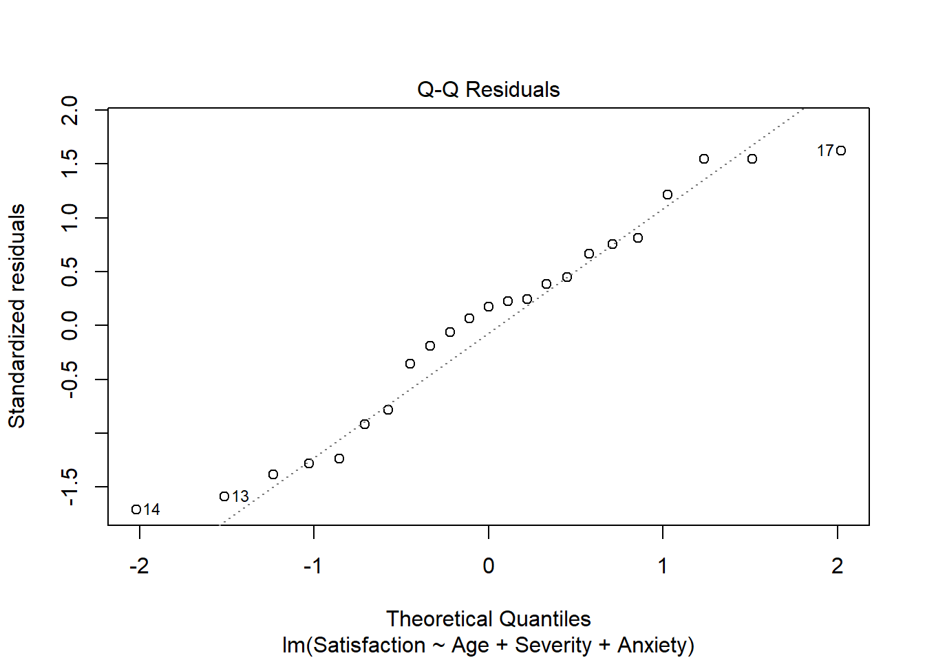
To check normality we look at the normal Q-Q plot of the residuals The data show departure from normality because the plot does not resemble a straight line. This departure could be due to the few observations. There are only 23 observations.
plot(res, 2)
Constant variance and Linearity
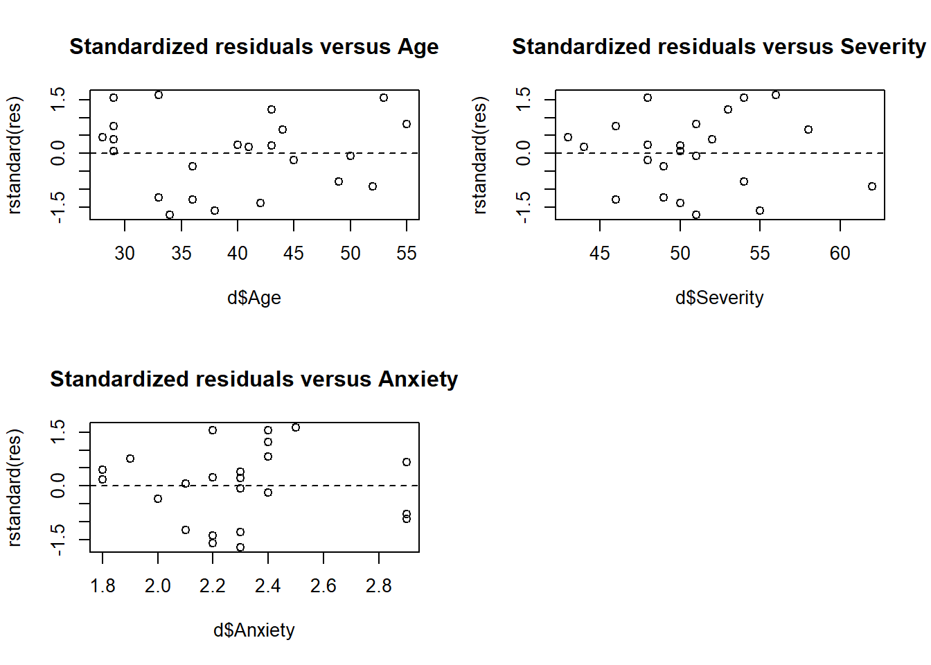
Constant variance. The plots suggest that the variance of \(y\), \(\sigma^2\), is the same for all values of \(x\) since we do not see any structure in the residuals.
Linearity. Residual versus variables plots are randomly scattered. This indicates that assuming the effects of age, severity and anxiety level are linear is OK.
par(mfrow =c(2, 2))plot(d$Age, rstandard(res), main ="Standardized residuals versus Age")abline(h =0, lty =2)plot(d$Severity, rstandard(res), main ="Standardized residuals versus Severity")abline(h =0, lty =2)plot(d$Anxiety, rstandard(res), main ="Standardized residuals versus Anxiety")abline(h =0, lty =2)
17.3 Unusual observations
Outliers (unusual \(y\)). Standardized residuals less than -2 or greater than 2.
# Outliersop <-which(abs(rstandard(res)) >2)op
named integer(0)
High leverage observations (unusual \(x\)). Leverage greater than 2 times the average of all leverage values. That is, \(h_{ii} > 2(p+1)/n\).
# High leverage observationsh <-hatvalues(res)lp <-which(h >2*length(res$coefficients)/nrow(d))lp
named integer(0)
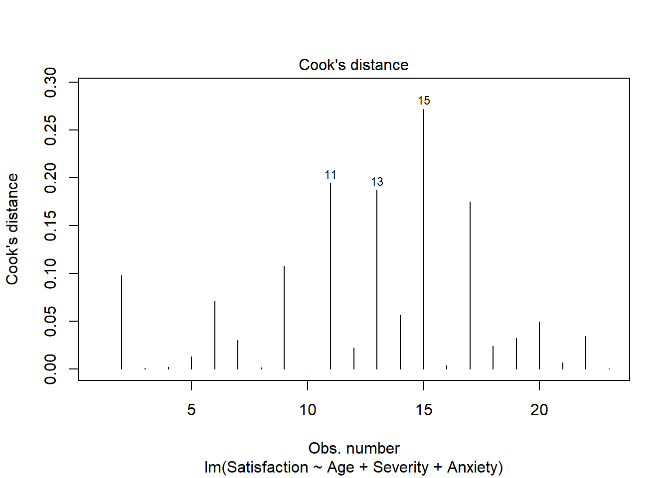
Influential values. Cook’s distance higher than \(4/n\).
There are not outliers or high leverage observations. Observations 11, 13, 15 and 17 have large Cook’s distance but it is not that different from the rest.