set.seed(4321)
x <- runif(200, min = 0, max = 4*pi)
x <- sort(x)
y <- sin(x) + rnorm(200, sd = 0.3)
plot(x, y, pch = 20)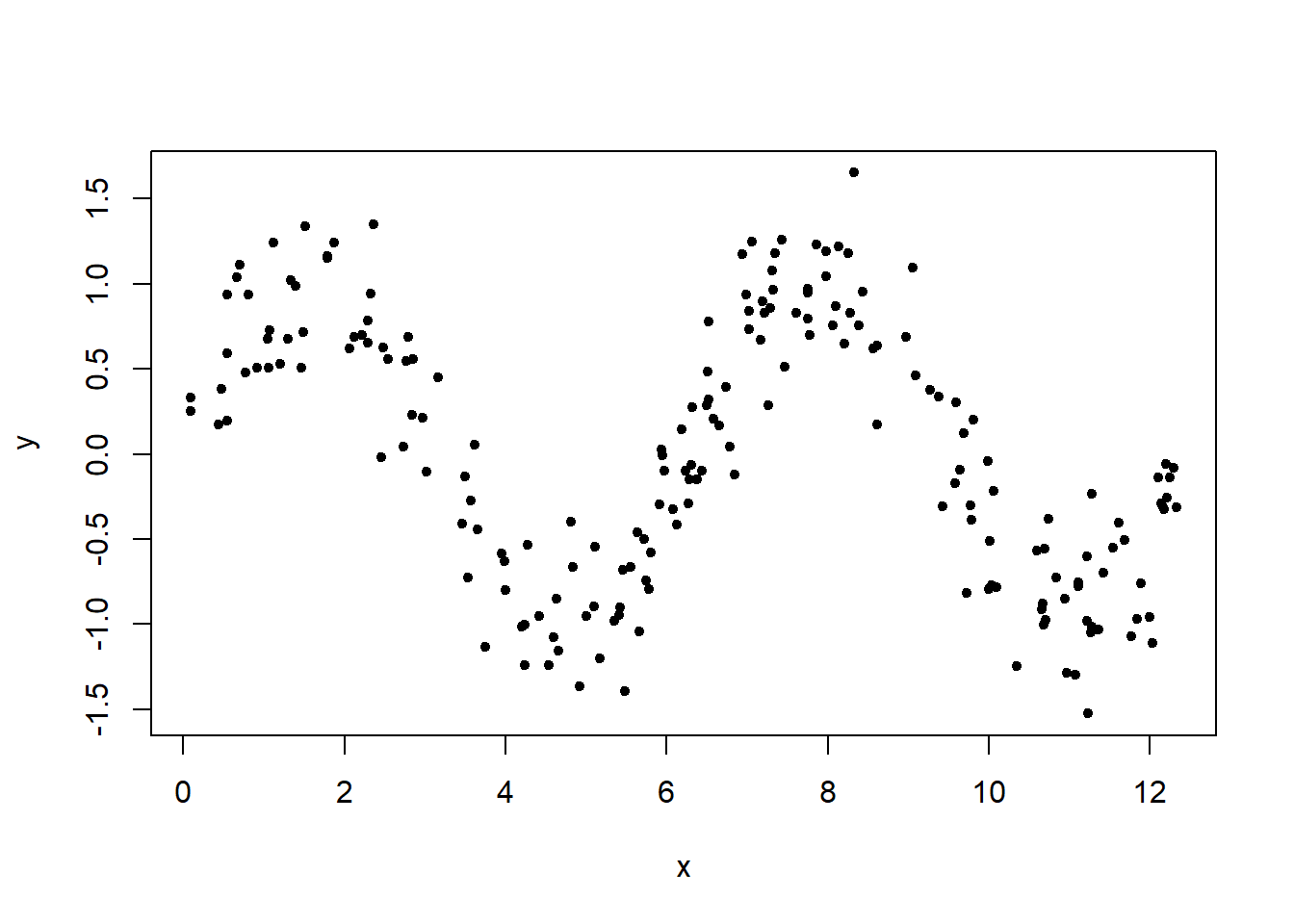
Estimating the effects of a covariate \(x\) on a response \(y\) non-parametrically, letting the data suggest the appropriate functional form.
Consider a linear model with one predictor
\[y = f(x) + \epsilon\]
We want to estimate \(f\), the trend or smooth. Assume data are ordered so \(x_1 < x_2 < \ldots < x_n\).
set.seed(4321)
x <- runif(200, min = 0, max = 4*pi)
x <- sort(x)
y <- sin(x) + rnorm(200, sd = 0.3)
plot(x, y, pch = 20)
fit <- lm(y ~ x)
plot(x, y, pch = 20)
abline(fit, lwd = 4, col = "red")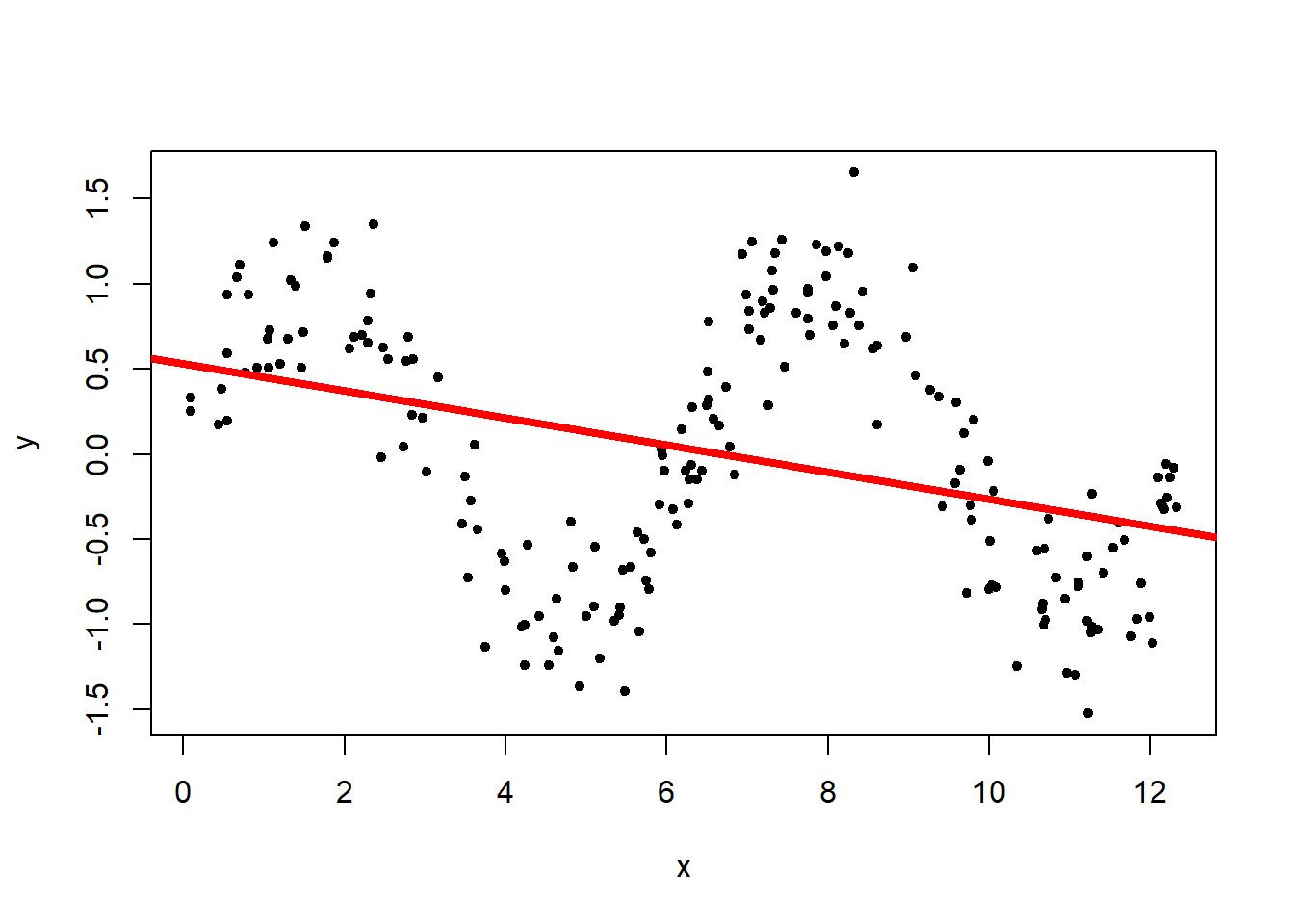
The linear regression (red line) does not capture the underlying structure. This is due to the fact that linear regression is only capable of detecting the linear relationship between the two variables. In this dataset, though, we can observe a clear relationship between \(x\) and \(y\) but they have a non-linear relationship, resulting in a bad outcome from the linear regression.
We estimate the smooth at \(x_i\) by averaging the \(y\)’s corresponding to \(x\)’s in a neighborhood of \(x_i\):
\[S(x_i) = \sum_{j \in N(x_i)} y_j/n_i\]
for a neighborhood \(N(x_i)\) with \(n_i\) observations. A common choice is to take a symmetric neighborhood consisting of the nearest \(2k+1\) points:
\[N(x_i)=\left( max(i-k,1), \ldots, i-1, i, i+1, min(i+k,n) \right)\]
library(zoo)
# k: integer width of the rolling window
# fill: vector with filling values at the left/within/to the right of the data range
plot(x, y, pch = 20)
lines(x, rollmean(y, k = 3, fill = c(NA, NULL, NA)), lwd = 4, col = "purple")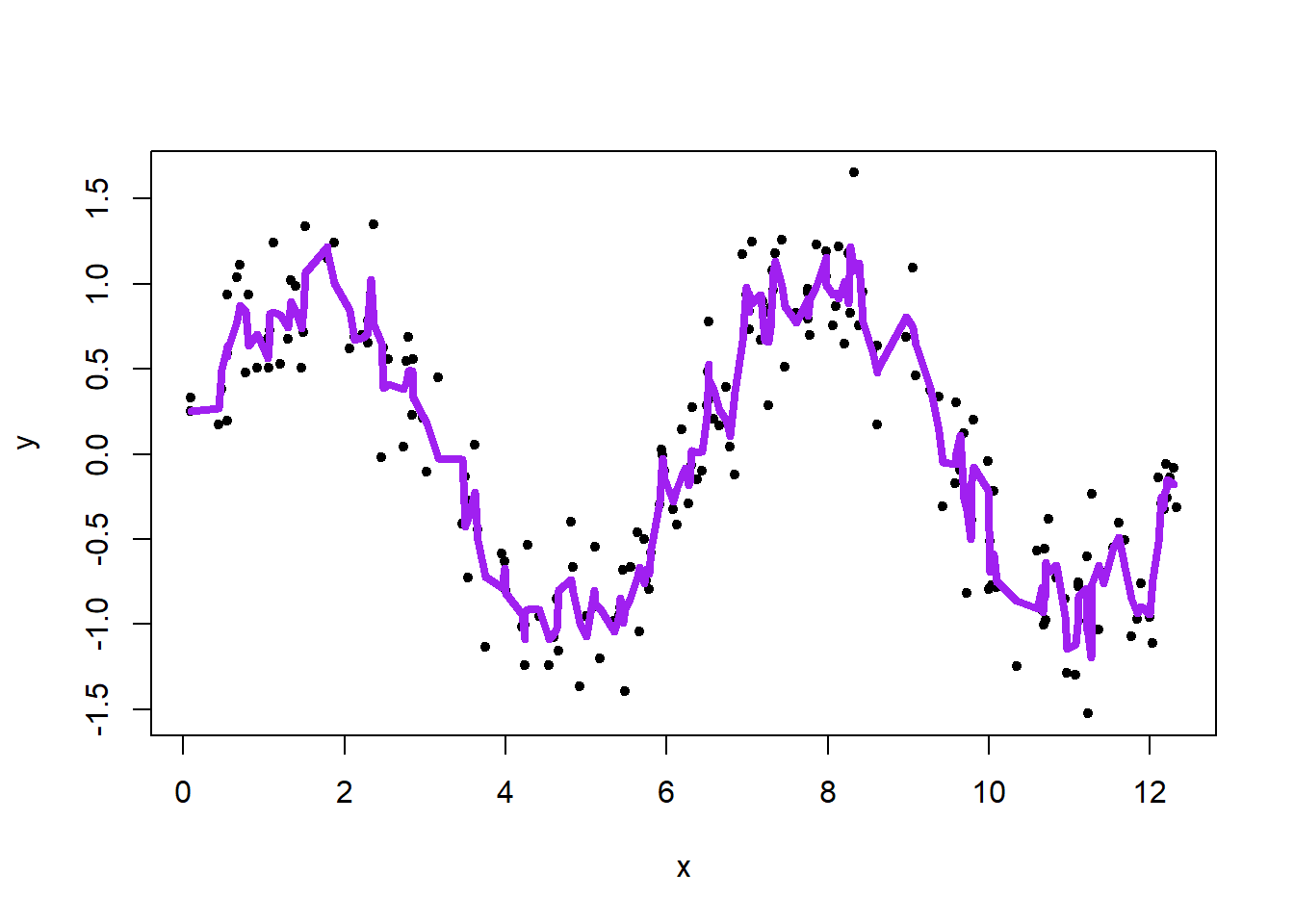
Curve is wiggly.
An alternative approach is to use a weighted running mean, with weights that decline as one moves away from the target value
\[S(x_i) = \sum_{j} w_{ij} y_j\]
To calculate \(S(x_i)\), the j-th point receives weight that can be calculated with a Kernel function.
\[w_{ij} = \frac{c_i}{\lambda}K\left( \frac{|x_i-x_j|}{\lambda} \right)\] where \(K(\cdot)\) is a symmetric function about the \(y\) axis \(K(-x) = K(x)\), \(\lambda\) is a tuning constant called the window width or bandwidth, and \(c_i\) is a normalizing constant so the weights add up to one for each \(x_i\).
The bandwidth \(\lambda\) determines the amount of smoothing applied in estimating \(f(x)\).
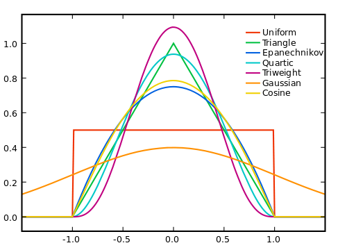
A kernel is a non-negative real-valued integrable function \(K\). For most applications, it is desirable to define the function to satisfy two additional requirements:
Popular choices of function \(K(\cdot)\) are:
When we set kernel = "normal", we are using the Gaussian function as the kernel. The argument bandwidth controls the amount of smoothing.
kreg <- ksmooth(x, y, kernel = "normal", bandwidth = 0.9)
plot(x, y, pch = 20)
lines(kreg, lwd = 4, col = "purple")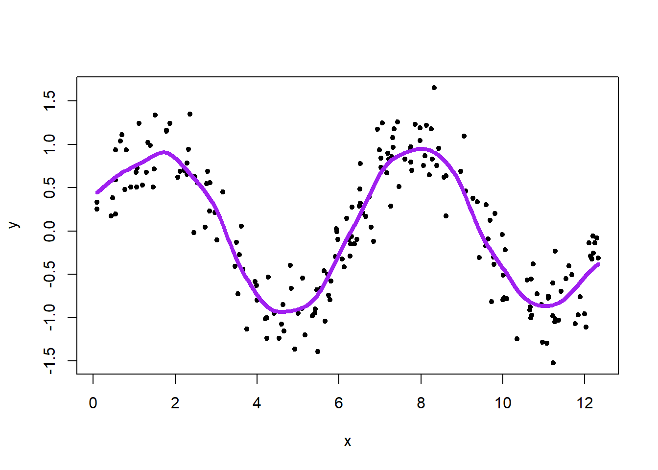
Here are examples of changing the value of bandwidth:
kreg1 <- ksmooth(x, y, kernel = "normal", bandwidth = 0.1)
kreg2 <- ksmooth(x, y, kernel = "normal", bandwidth = 0.9)
kreg3 <- ksmooth(x, y, kernel = "normal", bandwidth = 3.0)
plot(x, y, pch = 20)
lines(kreg1, lwd = 4, col = "orange")
lines(kreg2, lwd = 4, col = "purple")
lines(kreg3, lwd = 4, col = "limegreen")
legend("topright", c("h = 0.1", "h = 0.9", "h = 3.0"), lwd = 6, col = c("orange", "purple", "limegreen"))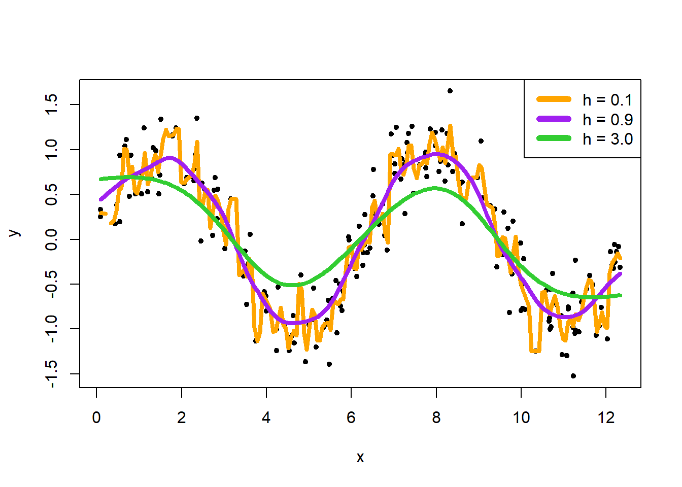
Fit kernel regression and choose the bandwidth using cross-validation.
set.seed(4321)
x <- runif(200, min = 0, max = 4*pi)
y <- sin(x) + rnorm(200, sd = 0.3)
plot(x, y, pch = 20)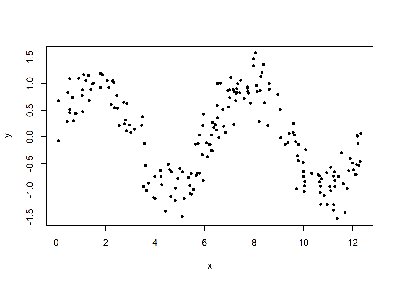
We can choose the bandwidth using leave-one-out cross-validation (LOOCV).
For bandwidth = 0.9. Prediction error is mean(CV_err)
fnloocv <- function(x, y, h){
# n sample size
n <- length(x)
CV_err = rep(NA, n)
for(i in 1:n){
# validation set
x_val <- x[i]
y_val <- y[i]
# training set
x_tr <- x[-i]
y_tr <- y[-i]
# we measure the error in terms of difference square
y_val_predict <- ksmooth(x = x_tr, y = y_tr, kernel = "normal", bandwidth = h, x.points = x_val)
CV_err[i] <- (y_val - y_val_predict$y)^2
}
return(mean(CV_err))
}

fnloocv(x, y, 0.9)
[1] 0.1027413Calculate prediction error for different values of \(h\) using LOOCV.
h_seq <- seq(from = 0.2, to = 2.0, by = 0.1)
# smoothing bandwidths we are using
CV_err_h <- rep(NA, length(h_seq))
for(j in 1:length(h_seq)){
CV_err_h[j] <- fnloocv(x, y, h_seq[j])
}

plot(h_seq, CV_err_h, type = "b", lwd = 3,
xlab = "Smoothing bandwidth", ylab = "LOOCV prediction error")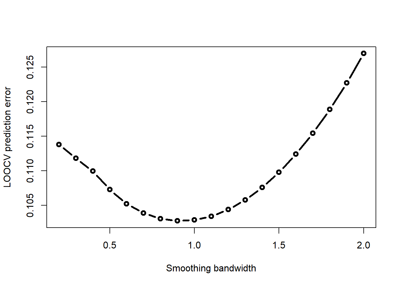
Choose the smoothing bandwidth that minimizes this LOOCV error
h_seq[which.min(CV_err_h)][1] 0.9\[Y_i = exp(-0.1 X_i) cos(X_i) + \epsilon_i,\ \ X_i \sim \mbox{Unif}[0, 6\pi],\ \ \epsilon \sim N(0, 0.1^2)\]
Show a scatter plot of \(X, Y\) and the fit of a kernel regression with smoothing bandwidth \(h=0.5\) and Gaussian kernel (kernel = "normal").
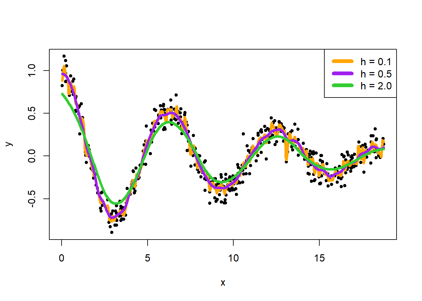
Consider three smoothing bandwidth \(h = 0.1, 0.5, 2.0\). Show the fit of the kernel regression to each of them. Which smoothing bandwidth seems to be the best one?
Use leave-one out cross-validation to show the smoothing bandwidth versus CV-error plot for the kernel regression. Which smoothing bandwidth provides you the minimal CV-error? (You could search in the range of \(h\) [0.1, 2.0])
set.seed(4321)
x <- sort(runif(500, 0, 6*pi))
y <- exp(-.1 * x) * cos(x) + rnorm(length(x), 0, sd = 0.1)
plot(x, y)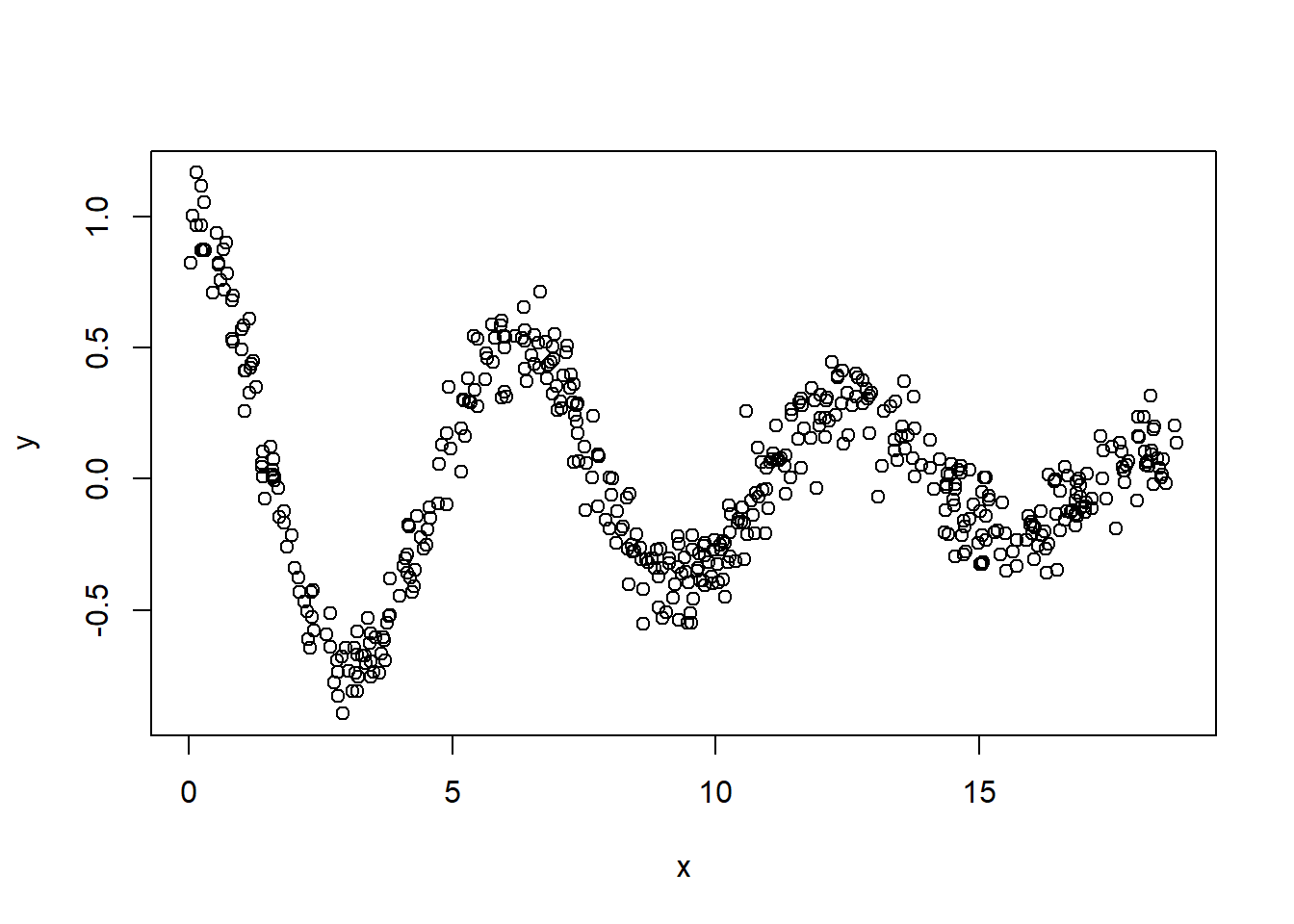
kreg1 <- ksmooth(x, y, kernel = "normal", bandwidth = 0.1)
kreg2 <- ksmooth(x, y, kernel = "normal", bandwidth = 0.5)
kreg3 <- ksmooth(x, y, kernel = "normal", bandwidth = 2.0)
plot(x, y, pch = 20)
lines(kreg1, lwd = 4, col = "orange")
lines(kreg2, lwd = 4, col = "purple")
lines(kreg3, lwd = 4, col = "limegreen")
legend("topright", c("h = 0.1", "h = 0.5", "h = 2.0"), lwd = 6, col = c("orange", "purple", "limegreen"))