set.seed(1974)
library(MultiKink)
library(ggplot2)
data("triceps") # load dataset triceps from MultiKink package

d <- triceps
d$x <- d$age
d$y <- d$triceps
g <- ggplot(d, aes(x, y)) + geom_point(alpha = 0.55, color = "black") + theme_minimal()
g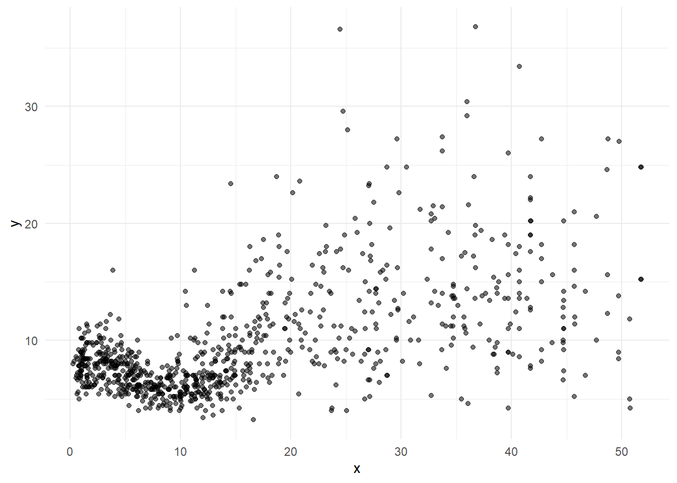
In the standard linear regression model, we assume that covariates have a linear effect on the response.
\[y_i = \beta_0 + \beta_1 x_i + \epsilon_i\]
Data from an study of 892 females under 50 years in three Gambian villages in West Africa. 892 observations with variables age (age of respondents), and triceps (triceps skinfold thickness).
set.seed(1974)
library(MultiKink)
library(ggplot2)
data("triceps") # load dataset triceps from MultiKink package
d <- triceps
d$x <- d$age
d$y <- d$triceps
g <- ggplot(d, aes(x, y)) + geom_point(alpha = 0.55, color = "black") + theme_minimal()
g
pred <- predict(lm(y ~ x, data = d))
g + geom_line(data = d, aes(x = x, y = pred), linewidth = 1, col="blue") 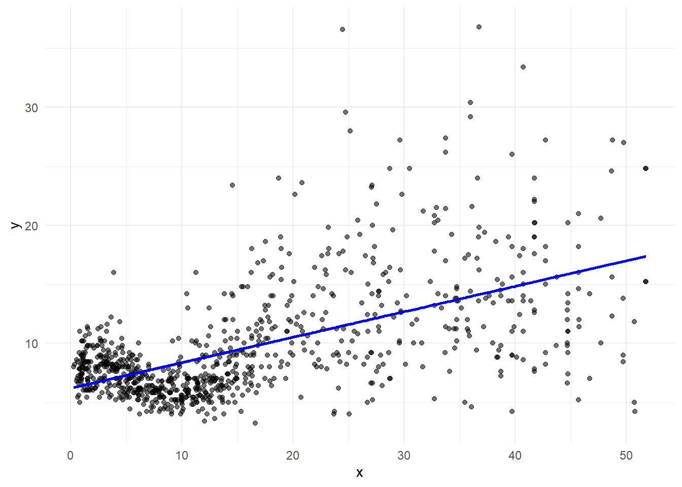
Here, we extend the standard linear regression model to settings in which the relationship between the predictors and the response is non-linear.
We model the response using a combination of basis functions. Basis functions are a family of functions or transformations that can be applied to a variable \(x\): \(b_1(x), b_2(x), \ldots, b_K(x)\).
\[y_i = \beta_0 + \beta_1 b_1(x_i) + \beta_2 b_2(x_i) + \beta_3 b_3 (x_i) + \ldots + \beta_K b_K(x_i) + \epsilon_i\]
We can consider this as a standard linear regression model with predictors \(b_1(x_i), \ldots, b_K(x_i)\) and use least squares to estimate the unknown regression coefficients.
Polynomial regression adds extra predictors obtained by raising each of the original predictors to a power. For example, a cubic regression uses three variables \(x\), \(x^2\), \(x^3\) as predictors.
Polynomial regression: basis functions are \(b_j(x_i) = x_i^j\)
Piecewise polynomials divide the range of the variable \(x\) into \(K\) distinct regions. Within each region, a polynomial function is fit to the data.
Piecewise constant functions: basis functions are \(b_j(x_i) = I(c_j \leq x_i \leq c_{j+1})\)
Regression splines divide the range of the variable \(x\) into \(K\) distinct regions. Within each region, a polynomial function is fit to the data. These polynomials are constrained so that they join smoothly at the regions boundaries or knots.
Regression splines: basis functions are truncated power functions \(b_j(x_i) = h_j(x_i)\)
Polynomial regression provides a simple way to provide a nonlinear fit to data.
Polynomial regression extends the linear model by adding extra predictors, obtained by raising each of the original predictors to a power.
\[y_i = \beta_0 + \beta_1 x_i + \beta_2 x_i^2 + \beta_3 x_i^3 + \ldots + \beta_d x_i^d + \epsilon_i\] For example, a cubic regression uses three variables, \(x\), \(x^2\), and \(x^3\) as predictors.
pred <- predict(lm(y ~ x + I(x^2) + I(x^3), data = d))
g + geom_line(data = d, aes(x = x, y = pred), linewidth = 1, col="blue")
For large regression enough degree \(d\), a polynomial regression allows us to produce an extremely non-linear curve.
Coefficients can be easily estimated using least squares linear regression because this is just a standard linear model with predictors \(x_i, x_i^2, \ldots, x_i^d\).
It is unusual to use \(d\) greater than 3 or 4 because for large values of \(d\), the polynomial curve can become overly flexible and can take on some very strange shapes. This is especially true near the boundary of the \(x\) variable.
Using polynomial functions of the variables as predictors in a linear model imposes a global structure of the non-linear function of \(x\) (each observation affects the entire curve, even for \(x\) values far from the observation)
Instead of fitting a high-degree polynomial over the entire range of \(x\), we can choose \(K\) knots, divide the range of \(x\) into \(K+1\) contiguous intervals and fit separate polynomials in each interval.
That is, we fit a polynomial model within the intervals defined by the knots.
\[y_i = \beta_0 + \beta_1 x_i + \beta_2 x_i^2 + \ldots + \beta_p x_i^p + \epsilon_i\]
where the coefficients \(\beta_0, \beta_1, \ldots, \beta_p\) differ in different parts of the range of \(x\). The points of the coefficients change are called knots. That is,
\[ \begin{array}{ll} y = \beta_0^{(1)} + \beta_1^{(1)}x + \ldots + \beta_p^{(1)}x^p + \epsilon^{(1)} & \mbox{for } x \leq K_1\\ y = \beta_0^{(2)} + \beta_1^{(2)}x + \ldots + \beta_p^{(2)}x^p+ \epsilon^{(2)} & \mbox{for } K_1 \leq x < K_2\\ \vdots & \vdots\\ y = \beta_0^{(K+1)} + \beta_1^{(K+1)}x + \ldots + \beta_p^{(K+1)}x^p + \epsilon^{(K+1)} & \mbox{for } K_K \leq x\\ \end{array} \]
# Function to plot variable and prediction in each interval
fnPlot <- function(g, pred1, pre2, pred3, pred4, pred5, pred6){
g + geom_line(data=d[d$x<5,], aes(y = pred1, x=age), linewidth = 1, col="blue") +
  geom_line(data=d[d$x >=5 & d$x<10,], aes(y = pred2, x=age), linewidth = 1, col="blue") +
  geom_line(data=d[d$x>=10 & d$x<20,], aes(y = pred3, x=age), linewidth = 1, col="blue") +
  geom_line(data=d[d$x>=20 & d$x<30,], aes(y = pred4, x=age), linewidth = 1, col="blue") +
  geom_line(data=d[d$x>=30 & d$x<40,], aes(y = pred5, x=age), linewidth = 1, col="blue") +
  geom_line(data=d[d$x>=40,], aes(y = pred6, x=age), linewidth = 1, col="blue")
}
Piecewise constant model (step functions)
Step function is a special case with polynomial of degree 0.
Choose knots \(c_1, c_2, \ldots, c_K\) in the range of \(x\) and then construct \(K+1\) new variables
\(C_0(x) = I(x < c_1)\)
\(C_1(x) = I(c_1 \leq x < c_2)\)
\(C_2(x) = I(c_2 \leq x < c_3)\)
\(\cdots\)
\(C_{K-1}(x) = I(c_{K-1} \leq x < c_K)\)
\(C_K(x) = I(c_K \leq x)\)
\[y_i = \beta_0 + \beta_1 C_1(x_i) + \beta_2 C_2(x_i) + \ldots + \beta_K C_K(x_i)+\epsilon_i\]
# Piecewise constant regression
pred1 <- mean(d[d$x < 5, ]$y)
pred2 <- mean(d[d$x >=5 & d$x<10,]$y)
pred3 <- mean(d[d$x>=10 & d$x<20,]$y)
pred4 <- mean(d[d$x>=20 & d$x<30,]$y)
pred5 <- mean(d[d$x>=30 & d$x<40,]$y)
pred6 <- mean(d[d$x>=40,]$y)

fnPlot(g, pred1, pre2, pred3, pred4, pred5, pred6)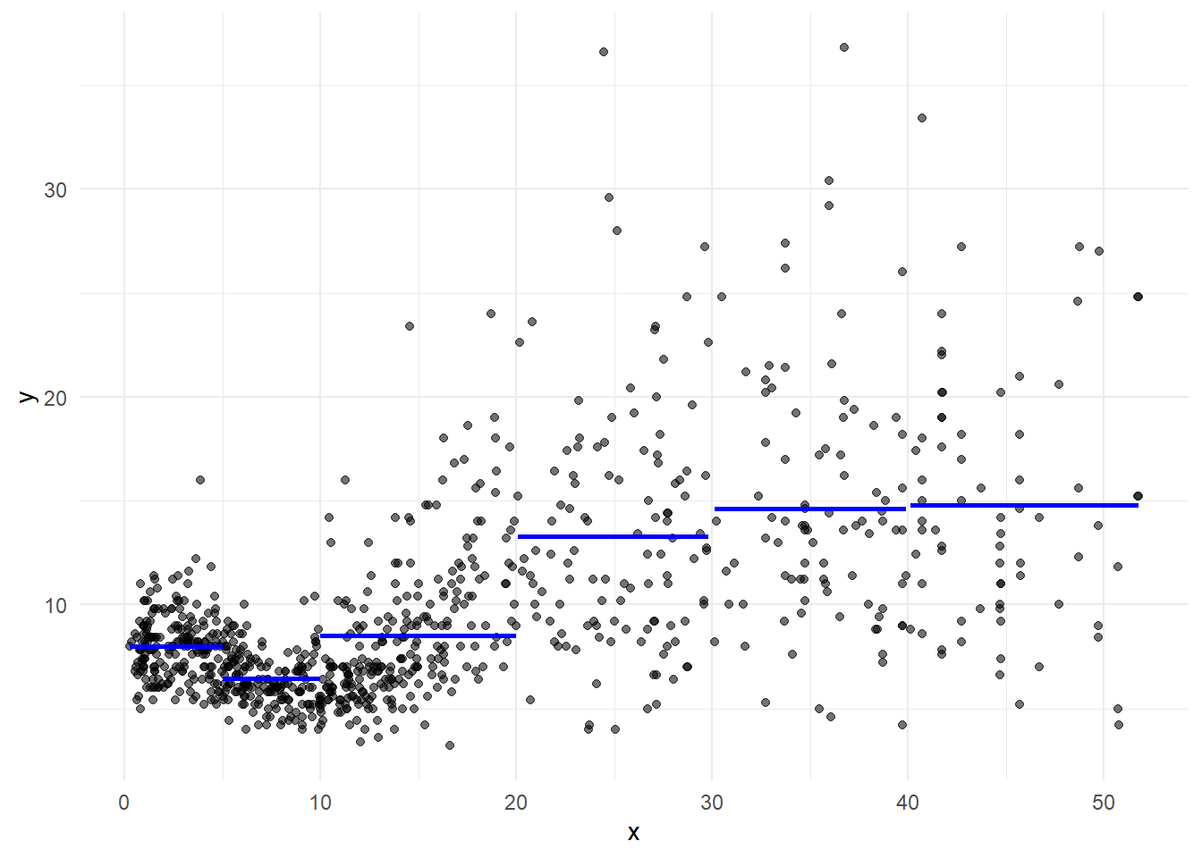
Piecewise linear model
# Piecewise linear regression
pred1 <- predict(lm(y ~ x, data = d[d$x < 5, ]))
pred2 <- predict(lm(y ~ x, data = d[d$x >= 5 & d$x < 10,]))
pred3 <- predict(lm(y ~ x, data = d[d$x >= 10 & d$x < 20,]))
pred4 <- predict(lm(y ~ x, data = d[d$x >= 20 & d$x < 30,]))
pred5 <- predict(lm(y ~ x, data = d[d$x >= 30 & d$x < 40,]))
pred6 <- predict(lm(y ~ x, data = d[d$x >= 40, ]))

fnPlot(g, pred1, pre2, pred3, pred4, pred5, pred6) 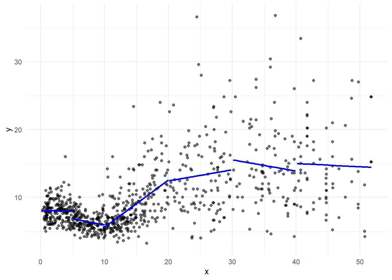
Piecewise cubic polynomial
# Piecewise cubic regression
pred1 <- predict(lm(y ~ x + I(x^2) + I(x^3), data = d[d$x < 5, ]))
pred2 <- predict(lm(y ~ x + I(x^2) + I(x^3), data = d[d$x >= 5 & d$x < 10,]))
pred3 <- predict(lm(y ~ x + I(x^2) + I(x^3), data = d[d$x >= 10 & d$x < 20,]))
pred4 <- predict(lm(y ~ x + I(x^2) + I(x^3), data = d[d$x >= 20 & d$x < 30,]))
pred5 <- predict(lm(y ~ x + I(x^2) + I(x^3), data = d[d$x >= 30 & d$x < 40,]))
pred6 <- predict(lm(y ~ x + I(x^2) + I(x^3), data = d[d$x >= 40, ]))

fnPlot(g, pred1, pre2, pred3, pred4, pred5, pred6) 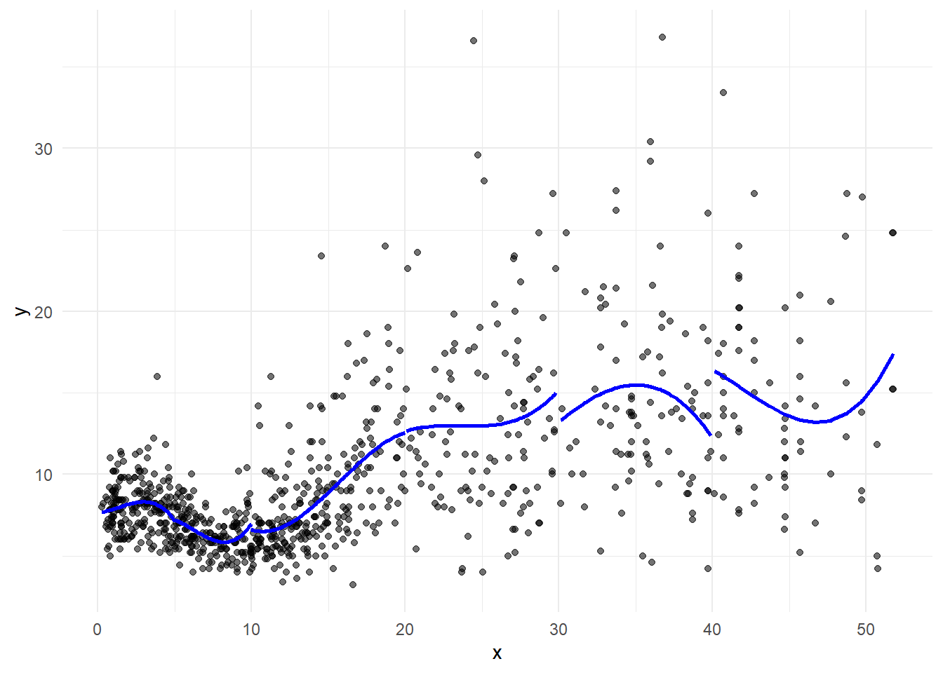
We can add constraints:
Continuous piecewise linear model
We can restrict the segments to be connected by including truncated power basis functions per knot.
\[y = \beta_0 + \beta_1 x + \beta_2 (x-5)_+ + \beta_3 (x-10)_+ \ \ldots + \beta_{5} (x-40)_+ + \epsilon\]
\[ (x-k)_+ = \left\{ \begin{array}{rl} 0 &\mbox{ if $x < k$} \\ x-k &\mbox{ if $x \geq k$} \end{array} \right. \]
x <- seq(0, 5, length.out = 200)
y1 <- (x-1)*I(x > 1)
y2 <- (x-3)*I(x > 3)

par(mfrow = c(1, 2))
plot(x, y1, type = "l", main = expression("k = 1, (x-1)"["+"]))
plot(x, y2, type = "l", main = expression("k = 3, (x-3)"["+"]))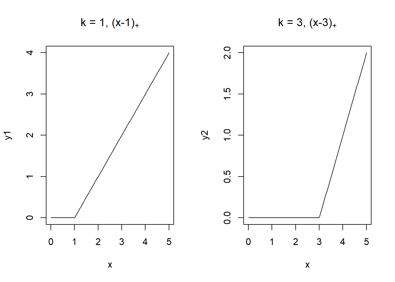
pred <- predict(lm(y ~ x + I((x-5)*(x>=5)) + I((x-10)*(x >= 10)) +
I((x-20)*(x >= 20)) + I((x-30)*(x >= 30)) + I((x-40)*(x >= 40)), data = d))

g + geom_line(data = d, aes(y = pred, x=x), linewidth = 1, col="blue") 
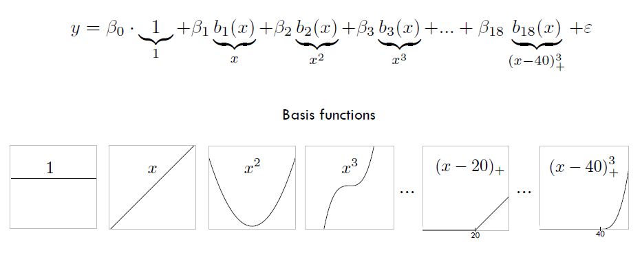
Continuous piecewise cubic model
We can restrict the polynomials to be connected by including truncated power basis functions per knot.
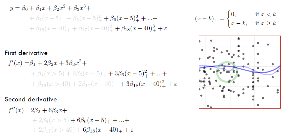
\[ \left\{ \begin{array}{rl} y = \beta_0 \ + & \beta_1 x + \beta_2 x^2 + \beta_3 x^3 +\\ + & \beta_4 (x-5)_+ + \beta_5 (x-5)^2_+ + \beta_5 (x-5)^3_+ \ldots +\\ + & \beta_{40} (x-40)_+ + \beta_{17} (x-40)^2_+ + \beta_{18} (x-40)^3_+ + \epsilon \end{array} \right. \]
\[ (x-k)_+ = \left\{ \begin{array}{rl} 0 &\mbox{ if $x < k$} \\ x-k &\mbox{ if $x \geq k$} \end{array} \right. \]
pred <- predict(lm(y ~ x + I(x^2) + I(x^3) +
I((x-5)*(x>=5)) + I((x-5)^2*(x>=5)) + I((x-5)^3*(x>=5)) +
I((x-10)*(x >= 10)) + I((x-10)^2*(x >= 10)) + I((x-10)^3*(x >= 10)) +
I((x-20)*(x >= 20)) + I((x-20)^2*(x >= 20)) + I((x-20)^3*(x >= 20)) +
I((x-30)*(x >= 30)) + I((x-30)^2*(x >= 30)) + I((x-30)^3*(x >= 30)) +
I((x-40)*(x >= 40)) + I((x-40)^2*(x >= 40)) + I((x-40)^3*(x >= 40)),
data = d))

g + geom_line(data = d, aes(y = pred, x=x), linewidth = 1, col="blue") 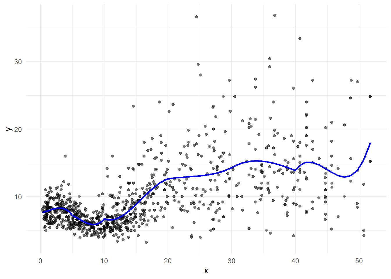
Piecewise cubic regression model is continuous at knots but does not have continuous first and second derivatives.

Cubic splines is continuous at knots and has continuous first and second derivatives.
\[ y = \beta_0 + \beta_1 x + \beta_2 x^2 + \beta_3 x^3 + \beta_5 (x-5)^3_+ \ldots + \beta_{8} (x-40)^3_+ + \epsilon \]
pred <- predict(lm(y ~ x + I(x^2) + I(x^3) +
I((x-5)^3*(x>=5)) +
I((x-10)^3*(x >= 10)) +
I((x-20)^3*(x >= 20)) +
I((x-30)^3*(x >= 30)) +
I((x-40)^3*(x >= 40)),
data = d))

g + geom_line(data = d, aes(y = pred, x=x), linewidth = 1, col="blue") 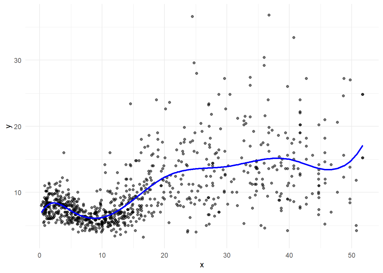
Regression splines of degree \(p\) are piecewise polynomials of degree \(p\) that have continuous derivatives up to order \(p-1\) at the knots.
Regression splines of degree \(p\) are piecewise polynomials of degree \(p\) joined together to make a single smooth curve.
Represent \(f(x)\) as a combination of \(1+p+K\) basis functions:
\[f(x) = \sum_{j=0}^{p+K} \beta_j h_j(x)\]
Start with a basis for a polynomial (\(1, x, x^2, \ldots, x^p\)) and then add one truncated power basis function per knot.
\[h_j(x) = x^{j}, j = 0, \ldots, p\]
\[h_{p+k_i}(x) = (x- k_i)_+^{p},\ i = 1, \ldots, K\]
\[ \begin{equation} h(x, k) = (x- k)_+^{p} = \begin{cases} 0 & \text{if $x < k$}\\ (x-k)^p & \text{if $x \geq k$} \end{cases} \end{equation} \]
To fit a regression spline of degree \(d\) and with \(K\) knots, we perform least squares regression with \(1+p+K\) parameters (an intercept and \(p+K\) predictors).
Cubic splines are piecewise cubic polynomials that are continuous and have continuous 1st and 2nd derivatives at the knots. Cubic splines are smooth at the knots.
A basis for a cubic spline consists of 1, \(x\), \(x^2\), \(x^3\) and one truncated power basis function per knot.
\[1, x, x^2, x^3, h(x, k_1), \dots, h(x,k_K).\] \[1, x, x^2, x^3, (x-k_1)_+^3, \dots, (x-k_K)_+^3.\]
A truncated power function for a knot \(k\) is a piecewise polynomial function with two pieces whose function values and derivatives of all orders up to \(p-1\) are zero at the knot.
\[ \begin{equation} h(x, k) = (x-k)_+^p = \begin{cases} 0 & \text{if $x < k$}\\ (x-k)^p & \text{if $x \geq k$} \end{cases} \end{equation} \]
\[ \begin{equation} h(x, k) = (x-k)_+^3 = \begin{cases} 0 & \text{if $x < k$}\\ (x-k)^3 & \text{if $x \geq k$} \end{cases} \end{equation} \]
x <- seq(0, 2, length.out = 200)
y1 <- (x-1)*I(x > 1)
y2 <- (x-1)^3*I(x > 1)

par(mfrow = c(1, 2))
plot(x, y1, type = "l", main = expression("linear (x-1)"["+"]))
plot(x, y2, type = "l", main = expression("cubic (x-1)"["+"]^3))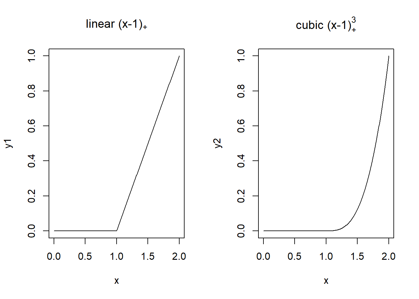
B-splines: The form of the truncated power basis leads to numerical instability. Powers of large numbers lead to rounding problems. B-splines provide an alternative, computationally convenient, and equivalent representation of the truncated power basis. B-spline representation is via a series of polynomial basis functions which have local support.
Natural splines: Regression splines can have high variance beyond the boundary knots. In particular, if there are few observations and/or knots close to the boundary. To “stabilize” the function near the boundaries, one can use natural splines. Natural spline is a regression spline with additional constraint that the function is linear beyond the boundary knots. This makes it more reliable in those regions.
Smoothing splines: Regression splines are created by specifying a set of knots, producing a sequence of basis functions, and then using least squares to estimate the spline coefficients. Choices regarding the number of knots and where they are located may have a large effect on the fit. Smoothing splines avoids the knot selection problem by using a maximal set of knots. The complexity of the fit is controlled by regularization. The smoothing spline is a natural cubic spline with knots at every unique value of \(x_i, i = 1, \ldots, n\). The penalty term translates to a penalty on the spline coefficients, which are shrunk some of the way toward the linear fit.