d <- read.table("data/pabmi.txt", header = TRUE)16 Example code SLR
16.1 BMI and physical activity study
- Researchers are interested in the relationship between physical activity (PA) measured with a pedometer and body mass index (BMI)
- A sample of 100 female undergraduate students were selected. Students wore a pedometer for a week and the average steps per day (in thousands) was recorded. BMI (kg/m\(^2\)) was also recorded.
- Is there a statistically significant linear relationship between physical activity and BMI? If so, what is the nature of the relationship?
Read data
Scatterplot of BMI versus PA
plot(d$PA, d$BMI)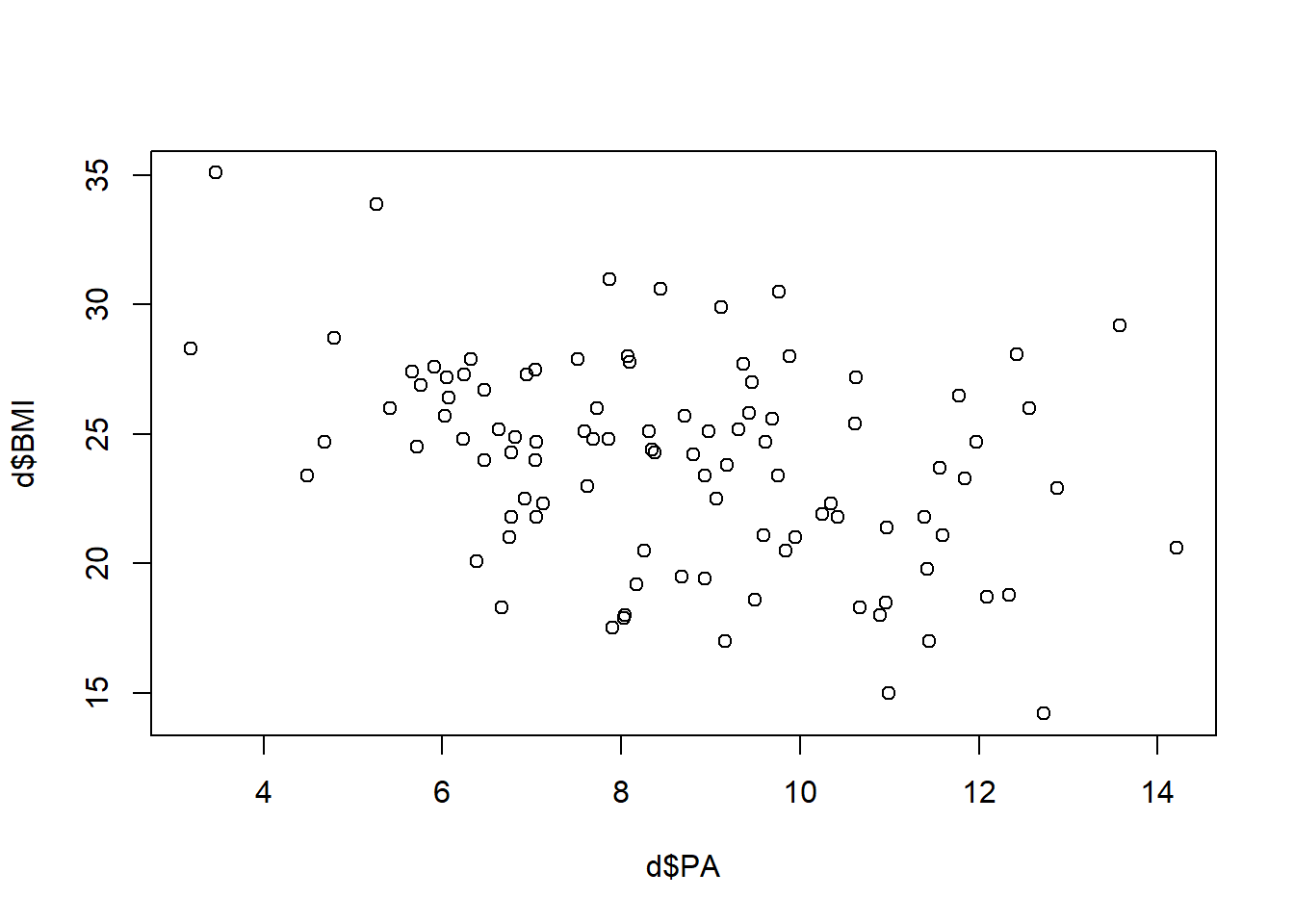
Model
\[Y_i = \beta_0 + \beta_1 X_{i} + \epsilon_i,\ \ \epsilon_i \sim^{iid} N(0, \sigma^2),\ \ \ i = 1,\ldots,n.\]
res <- lm(BMI ~ PA, data = d)
summary(res)
Call:
lm(formula = BMI ~ PA, data = d)

Residuals:
    Min      1Q  Median      3Q     Max
-7.3819 -2.5636  0.2062  1.9820  8.5078

Coefficients:
            Estimate Std. Error t value Pr(>|t|)
(Intercept)  29.5782     1.4120  20.948  < 2e-16 ***
PA           -0.6547     0.1583  -4.135  7.5e-05 ***
---
Signif. codes:  0 '***' 0.001 '**' 0.01 '*' 0.05 '.' 0.1 ' ' 1

Residual standard error: 3.655 on 98 degrees of freedom
Multiple R-squared:  0.1485,    Adjusted R-squared:  0.1399
F-statistic:  17.1 on 1 and 98 DF,  p-value: 7.503e-05
16.2 Checking assumptions linear model
Independency
Independency: data are randomly collected, observations are independent
Normality
Normality: in the normal Q-Q plot points lie close to the straight line
A Q-Q plot compares the data with what to expect to get if the theoretical distribution from which the data come is normal.
The Q-Q plot displays the value of observed quantiles in the standardized residual distribution on the y-axis versus the quantiles of the theoretical normal distribution on the x-axis.
- If data are normally distributed, we should see the plotted points lie close to the straight line.
- If we see a concave normal probability plot, log transforming the response variable may remove the problem.
plot(res, 2)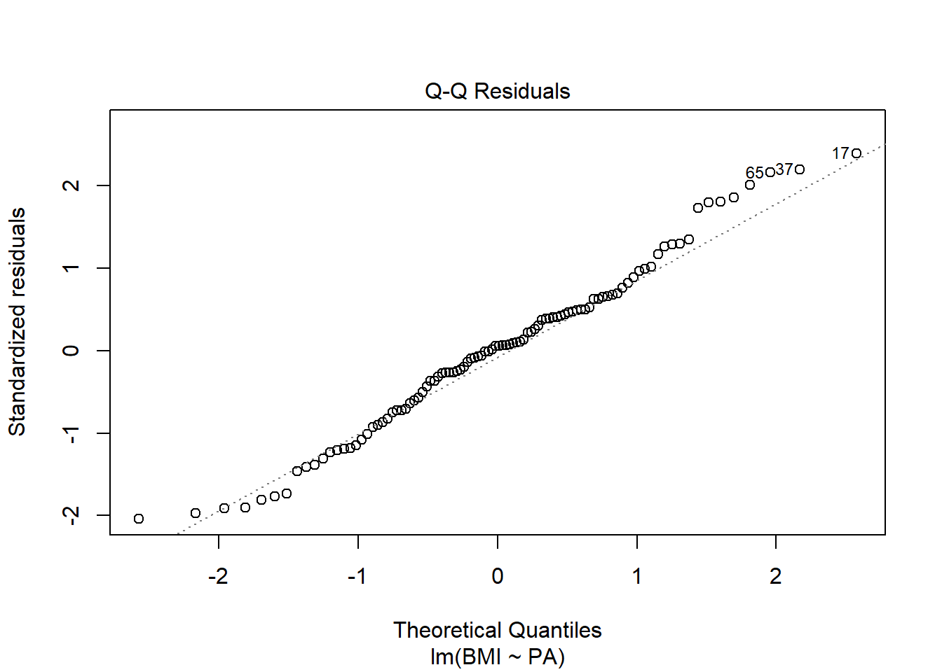
Constant variance
Constant variance: residual vs fits plots are randomly scattered around 0
plot(res, 1)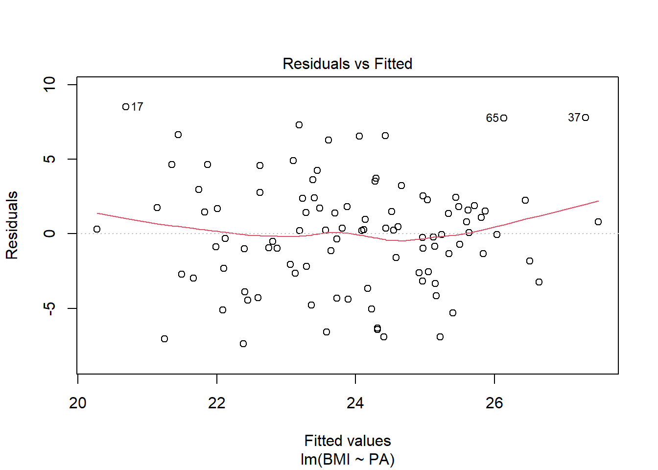
Linearity
Linearity: residual vs fits plots are randomly scattered around 0
plot(res, 1)
16.3 Unusual observations
Outliers (unusual \(y\)). Standardized residuals less than -2 or greater than 2.
# Outliers
op <- which(abs(rstandard(res)) > 2)
op
1 17 37 65 89
1 17 37 65 89 plot(d$PA, d$BMI)
text(d$PA[op], d$BMI[op]-.5, paste("outlier", op))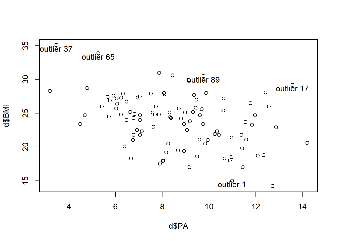
High leverage observations (unusual \(x\)). Leverage greater than 2 times the average of all leverage values. That is, \(h_{ii} > 2(p+1)/n\).
# High leverage observations
h <- hatvalues(res)
lp <- which(h > 2*length(res$coefficients)/nrow(d))
lp
6 17 37 59 79 83 85
6 17 37 59 79 83 85 plot(d$PA, d$BMI)
text(d$PA[lp], d$BMI[lp]-.5, paste("lev", lp))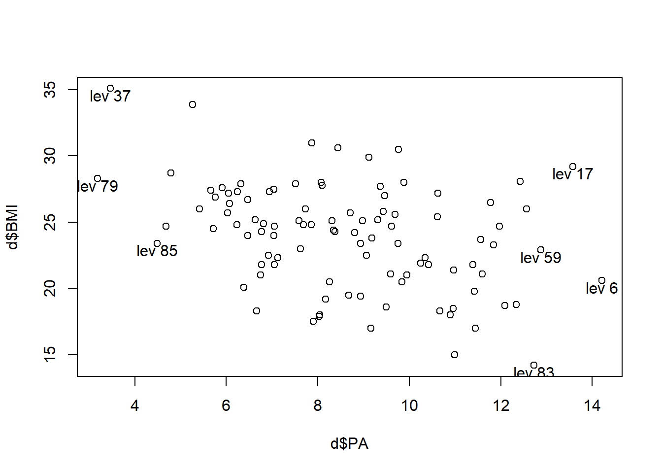
Influential values. Cook’s distance higher than \(4/n\).
Cook’s distance combines residuals and leverages in a single measure of influence. We should examine in closer detail the points with values Cook’s distance that are substantially larger than the rest (17 and 37).
# Influential observations
ip <- which(cooks.distance(res) > 4/nrow(d))
ip
1 3 17 37 65 83
1 3 17 37 65 83 plot(d$PA, d$BMI)
text(d$PA[ip], d$BMI[ip]-.5, paste("infl", ip))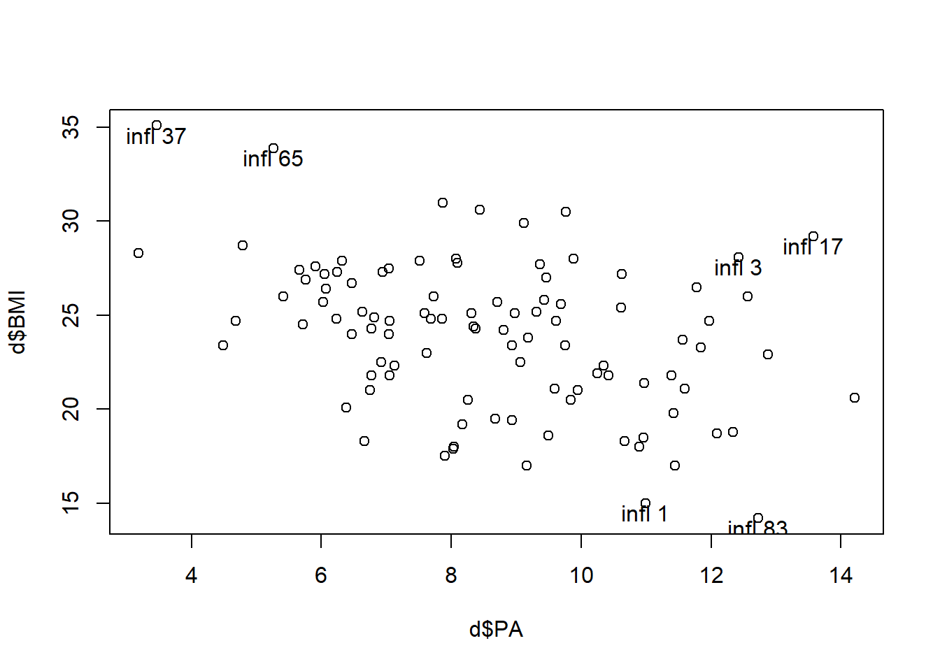
plot(res, 4)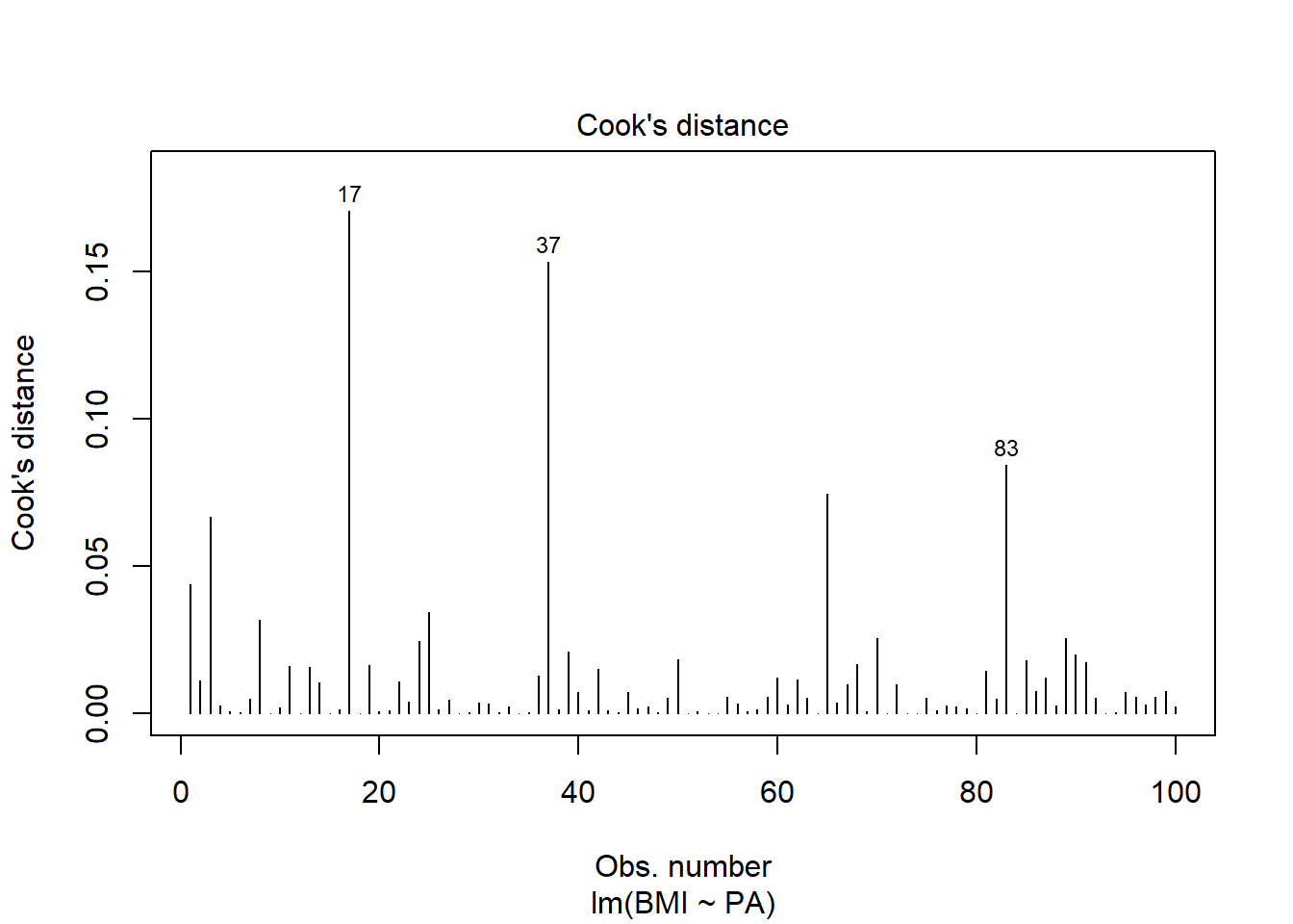
Standardized residuals versus leverage values
plot(res, 5)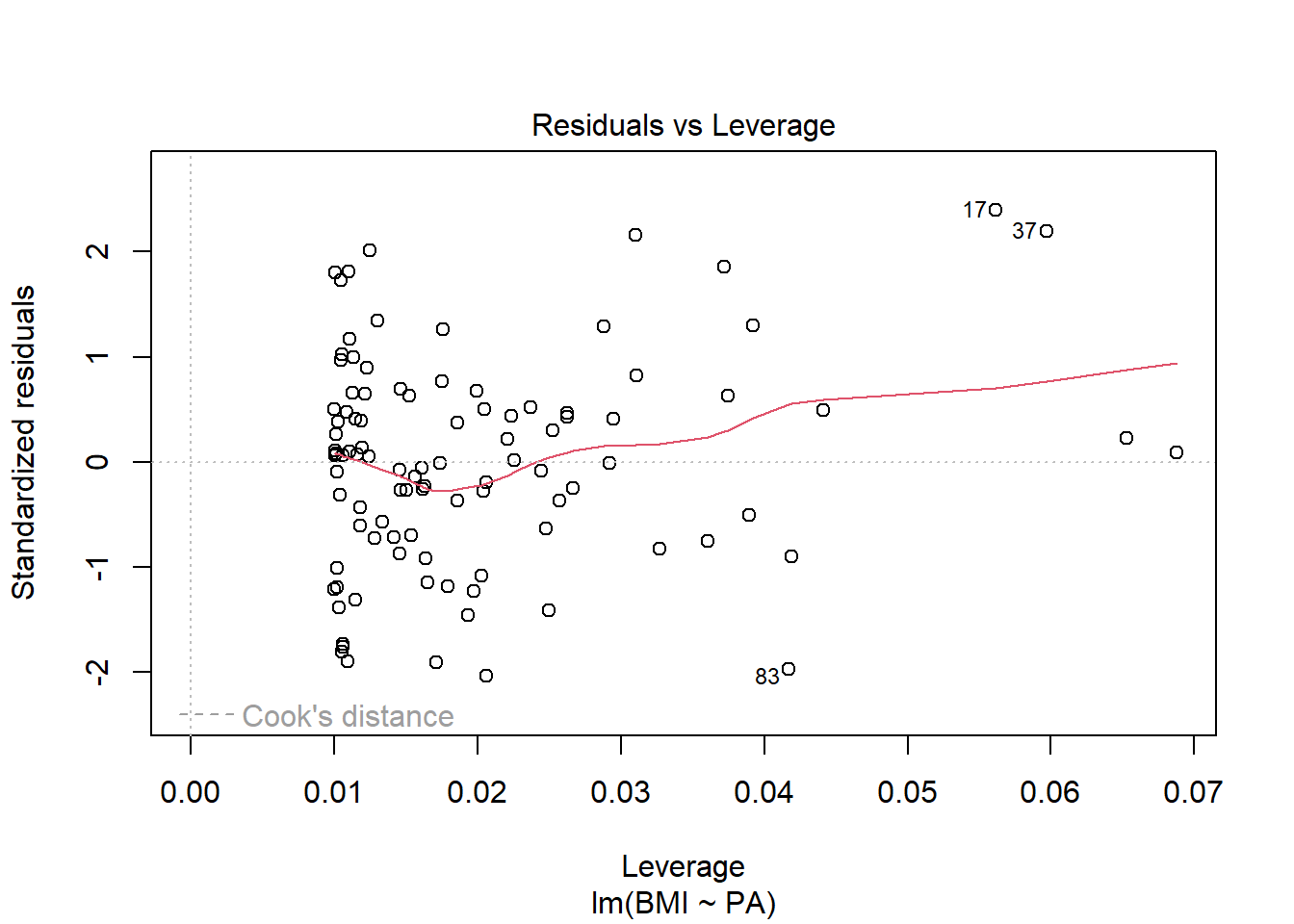
d[unique(c(lp, op, ip)), ] SUBJECT PA BMI
6 6 14.209 20.6
17 17 13.573 29.2
37 37 3.468 35.1
59 59 12.879 22.9
79 79 3.186 28.3
83 83 12.725 14.2
85 85 4.490 23.4
1 1 10.992 15.0
65 65 5.266 33.9
89 89 9.760 30.5
3 3 12.423 28.1