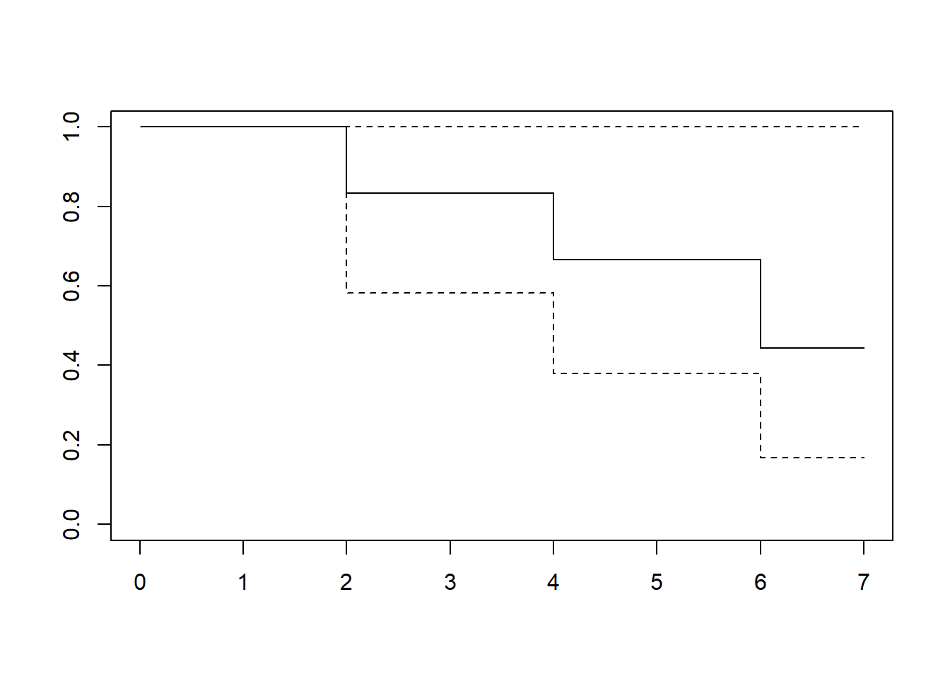
If we assume that every subject follows the same survival function (no covariates or other individual differences), we can easily estimate the survival function \(S(t)\) non-parametrically using the Kaplan-Meier (or product-limit) method.
The median survival time is the smallest \(t\) such that the survival function is less than or equal to 0.5: \(\hat t_{med} = \mbox{inf}\left\{t:\hat S(t) \leq 0.5 \right\}\).
\(P(A \mbox{ and } B) = P(B) = P(T > t(f)) = S(t(f))\)
\(t(f)\) is the next failure time after \(t(f-1)\) so there cannot be failures after \(t(f-1)\) and before time \(t(f)\). Since there are not failures during \(t(f-1) < T < t(f)\), then \(A = T \geq t(f)\) is \(A = T > t(f-1)\)
\(S(t(f)) = S(t(f-1)) \times P(T > t(f)| T \geq t(f))\)
27.2 Example
lung cancer data in the survival package.
inst: Institution code
time: Survival time in days
status: censoring status 1=censored, 2=dead
age: Age in years
sex: Male=1 Female=2
ph.ecog: ECOG performance score as rated by the physician. 0=asymptomatic, 1= symptomatic but completely ambulatory, 2= in bed <50% of the day, 3= in bed > 50% of the day but not bedbound, 4 = bedbound ph.karno: Karnofsky performance score (bad=0-good=100) rated by physician
pat.karno: Karnofsky performance score as rated by patient
meal.cal: Calories consumed at meals
wt.loss: Weight loss in last six months
library(survival)data("lung")
Warning in data("lung"): data set 'lung' not found
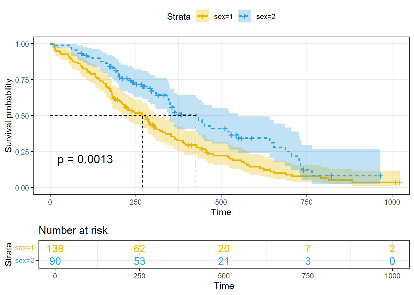
Computing survival curves with the survfit() function of the survival package.
fit <-survfit(Surv(time, status) ~ sex, data = lung)
Visualizing survival curves with the ggsurvplot() function of the survminer package.
library(survminer)# Change color, linetype by strata, risk.table color by strataggsurvplot(fit,pval =TRUE, conf.int =TRUE,risk.table =TRUE, # Add risk tablerisk.table.col ="strata", # Change risk table color by groupslinetype ="strata", # Change line type by groupssurv.median.line ="hv", # Specify median survivalggtheme =theme_bw(), # Change ggplot2 themepalette =c("#E7B800", "#2E9FDF"))
The log-rank test can be used to compare survival curves.