7 Linear regression model
7.1 Linear model
\[ \begin{matrix} Y_i = & \beta_0 + \beta_1 X_{i,1} + \beta_2 X_{i,2} + \ldots + \beta_p X_{i,p} + \epsilon_i, & i = 1,\ldots,n\\ & & \\ Y_1 = & \beta_0 + \beta_1 X_{1,1} + \beta_2 X_{1,2} + \ldots + \beta_p X_{1,p} + \epsilon_1 & \\ Y_2 = & \beta_0 + \beta_1 X_{2,1} + \beta_2 X_{2,2} + \ldots + \beta_p X_{2,p} + \epsilon_2 & \\ & \vdots & \\ Y_n = &\beta_0 + \beta_1 X_{n,1} + \beta_2 X_{n,2} + \ldots + \beta_p X_{n,p} + \epsilon_n & \\ \end{matrix} \]
where the error \(\epsilon_i\) is a Gaussian random variable with expectation zero and variance \(\sigma^2\), \(\epsilon_i \sim^{iid} N(0, \sigma^2)\).
\[E[Y_i] = \beta_0 + \beta_1 X_{i1} + \beta_2 X_{i2} + \ldots + \beta_p X_{ip},\ Var[Y_i]=\sigma^2, \ i = 1,\ldots,n\]
7.2 Linear model in matrix form
\[ \begin{matrix} \begin{bmatrix} Y_1 \\ Y_2 \\ \vdots \\ Y_n \\ \end{bmatrix} = & \begin{bmatrix} \beta_0 + \beta_1 X_{1,1} + \beta_1 X_{1,2} + \dots + \beta_p X_{1,p} \\ \beta_0 + \beta_1 X_{2,1} + \beta_1 X_{2,2} + \dots + \beta_p X_{2,p} \\ \vdots \\ \beta_0 + \beta_1 X_{n,1} + \beta_1 X_{n,2} + \dots + \beta_p X_{n,p} \\ \end{bmatrix} & + \begin{bmatrix} \epsilon_1 \\ \epsilon_2 \\ \vdots \\ \epsilon_n \\ \end{bmatrix} \\ & & \\ \begin{bmatrix} Y_1 \\ Y_2 \\ \vdots \\ Y_n \\ \end{bmatrix} = & \begin{bmatrix} 1 & X_{1,1} & X_{1,2} & \dots & X_{1,p}\\ 1 & X_{2,1} & X_{2,2} & \dots & X_{2,p}\\ \vdots \\ 1 & X_{n,1} & X_{n,2} & \dots & X_{n,p}\\ \end{bmatrix} \begin{bmatrix} \beta_0 \\ \beta_1 \\ \vdots \\ \beta_p \\ \end{bmatrix} & + \begin{bmatrix} \epsilon_1 \\ \epsilon_2 \\ \vdots \\ \epsilon_n \\ \end{bmatrix} \\ \end{matrix} \] \[\boldsymbol{Y} = \boldsymbol{X} \boldsymbol{\beta} + \boldsymbol{\epsilon}\]
- \(\boldsymbol{Y}\) is the response vector
- \(\boldsymbol{X}\) is the design matrix
- \(\boldsymbol{\beta}\) is the vector of parameters
- \(\boldsymbol{\epsilon}\) is the error vector
7.3 Covariance matrix of \(\boldsymbol{\epsilon}\) and \(\boldsymbol{Y}\)
\[ Cov[\boldsymbol{\epsilon}] = Cov \begin{bmatrix} \epsilon_1 \\ \epsilon_2 \\ \vdots \\ \epsilon_n \\ \end{bmatrix} = \begin{bmatrix} \sigma^2 & 0 & \dots & 0 \\ 0 & \sigma^2 & \dots & 0 \\ \vdots & \vdots & \ddots & \vdots \\ 0 & 0 & \dots & \sigma^2 \\ \end{bmatrix} = \sigma^2 \boldsymbol{I}_{n\times n} \]
\[ Cov[\boldsymbol{Y}] = Cov\begin{bmatrix} Y_1 \\ Y_2 \\ \vdots \\ Y_n \\ \end{bmatrix} = \begin{bmatrix} \sigma^2 & 0 & \dots & 0 \\ 0 & \sigma^2 & \dots & 0 \\ \vdots & \vdots & \ddots & \vdots \\ 0 & 0 & \dots & \sigma^2 \\ \end{bmatrix} = \sigma^2 \boldsymbol{I}_{n\times n} \]
In matrix form: \[\boldsymbol{Y} \sim N(\boldsymbol{X\beta}, \sigma^2 \boldsymbol{I})\]
7.4 Parameter estimation \(\boldsymbol{\hat \beta}\)
\(\boldsymbol{\epsilon} = \boldsymbol{Y} - \boldsymbol{X \beta}\).
Using least squares, we want to minimize sum of squared residuals
\[ \sum \epsilon_i^2 = \begin{bmatrix} \epsilon_1 & \epsilon_2 & \dots \epsilon_n \end{bmatrix} \begin{bmatrix} \epsilon_1 \\ \epsilon_2 \\ \vdots \\ \epsilon_n \\ \end{bmatrix} = \boldsymbol{\epsilon}' \boldsymbol{\epsilon} \]
In least squares estimation, we find the coefficients \(\boldsymbol{\beta}\) that minimize the residual sum of squares.
\[RSS(\boldsymbol{\beta}) = \sum_{i=1}^n\left(Y_i-\sum_{j=0}^p \beta_j X_{ij}\right)^2\]
\[RSS(\boldsymbol{\beta}) = \boldsymbol{\epsilon}' \boldsymbol{\epsilon} = (\boldsymbol{Y}-\boldsymbol{X\beta})'(\boldsymbol{Y}-\boldsymbol{X\beta})\] We take the derivative with respect to the vector \(\boldsymbol{\beta}\) \[ \frac{\partial RSS}{\partial \boldsymbol{\beta}} = - 2\boldsymbol{X'} (\boldsymbol{Y}-\boldsymbol{X\beta}) \]
\[\frac{\partial^2 RSS}{\partial \boldsymbol{\beta} \partial \boldsymbol{\beta}'} = 2 \boldsymbol{X'X}\]
Assuming that \(\boldsymbol{X}\) has full rank and hence \(\boldsymbol{X'X}\) is positive definite. We set the first derivative to zero and solve for \(\boldsymbol{\beta}\)
\[\boldsymbol{X}' (\boldsymbol{Y}-\boldsymbol{X\beta})=\boldsymbol{0}\]
\[\boldsymbol{X'Y} = (\boldsymbol{X'X}) \boldsymbol{\hat \beta} \mbox{ (Normal equations)}\]
\[\boldsymbol{\hat \beta} = \boldsymbol{(X'X)^{-1}X' Y}\]
7.5 Fitted values
\[ \boldsymbol{\hat Y} = \begin{bmatrix} \hat Y_1 \\ \hat Y_2 \\ \vdots \\ \hat Y_n \\ \end{bmatrix} = \begin{bmatrix} \hat \beta_0 + \hat \beta_1 X_{1,1} + \hat \beta_2 X_{1,2} + \dots + \hat \beta_p X_{1,p} \\ \hat \beta_0 + \hat \beta_1 X_{2,1} + \hat \beta_2 X_{2,2} + \dots + \hat \beta_p X_{2,p} \\ \vdots \\ \hat \beta_0 + \hat \beta_1 X_{n,1} + \hat \beta_2 X_{n,2} + \dots + \hat \beta_p X_{n,p} \\ \end{bmatrix} = \begin{bmatrix} 1 & X_{1,1} & X_{1,2} & \dots & X_{1,p} \\ 1 & X_{2,1} & X_{2,2} & \dots & X_{2,p} \\ \vdots & \vdots \\ 1 & X_{n,1} & X_{n,2} & \dots & X_{n,p} \\ \end{bmatrix} \begin{bmatrix} \hat \beta_0 \\ \hat \beta_1 \\ \vdots \\ \hat \beta_p \\ \end{bmatrix} = \boldsymbol{X \hat \beta} \]
\[\boldsymbol{\hat Y} = \boldsymbol{X \hat \beta} = \boldsymbol{X} (\boldsymbol{X'X})^{-1} \boldsymbol{X' Y} = \boldsymbol{H Y}\]
7.6 Hat matrix
\(\boldsymbol{H} =\boldsymbol{X}(\boldsymbol{X'X})^{-1} \boldsymbol{X'}\) is called hat matrix (\(\boldsymbol{H}\) puts a hat on \(\boldsymbol{Y}\)).
Residuals \(\boldsymbol{Y}- \boldsymbol{ \hat Y} = \boldsymbol{Y} - \boldsymbol{HY} = (\boldsymbol{I} - \boldsymbol{H}) \boldsymbol{Y}\)
\(\boldsymbol{H}\) and \((\boldsymbol{I}-\boldsymbol{H})\) are symmetric and idempotent:
Symmetric: \(\boldsymbol{H} = \boldsymbol{H'}\) and \((\boldsymbol{I}-\boldsymbol{H})' = (\boldsymbol{I}-\boldsymbol{H})\)
Idempotent: \(\boldsymbol{H}^2 = \boldsymbol{H}\) and \((\boldsymbol{I}-\boldsymbol{H})(\boldsymbol{I}-\boldsymbol{H}) = (\boldsymbol{I}-\boldsymbol{H})\)
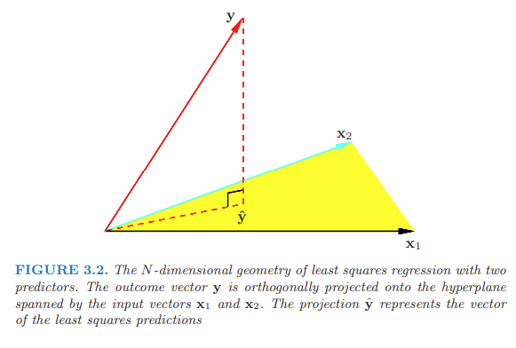
7.7 Geometrical interpretation of the least squares estimate
The least squares estimate \(\boldsymbol{\hat Y}\) is an element of the column space of \(\boldsymbol{X}\), the subspace of \(\mathbb{R}^n\) spanned by the column vectors of \(\boldsymbol{X}\) (\(\boldsymbol{X_0}, \boldsymbol{X_1} \ldots, \boldsymbol{X_p}\), with \(\boldsymbol{X_0}\) vector of 1s).
We obtain \(\boldsymbol{\hat Y}\) by minimizing the distance between \(\boldsymbol{Y}\) and \(\boldsymbol{\hat Y}\). That is, we minimize \(RSS(\boldsymbol{\beta}) = ||\boldsymbol{Y − X \beta}||^2\). So we choose \(\boldsymbol{\hat \beta}\) so that the residual vector \(\boldsymbol{Y - \hat Y}\) is orthogonal to the column space. This orthogonality is expressed in \(\boldsymbol{X'(Y-X \beta)}=\boldsymbol{0}\), and the resulting estimate \(\boldsymbol{\hat Y}\) is hence the orthogonal projection of \(\boldsymbol{Y}\) onto this subspace.
\(\boldsymbol{\hat Y} = \boldsymbol{X (X'X)^{-1}X' Y} = \boldsymbol{H Y}\). The hat matrix \(\boldsymbol{H}\) computes the orthogonal projection of \(\boldsymbol{Y}\), and hence it is also known as a projection matrix.
7.8 Distribution of \(\boldsymbol{\hat \beta}\)
\[\boldsymbol{\hat \beta} \sim N(\boldsymbol{\beta}, \sigma^2 \boldsymbol{(X'X)^{-1}})\]
Proof:
We know that \(\boldsymbol{\hat \beta} = \boldsymbol{(X'X)^{-1}} \boldsymbol{X' Y}\) and \(\boldsymbol{Y} \sim N(\boldsymbol{X \beta}, \sigma^2 \boldsymbol{I})\).
Since the only random variable involved in the expression of \(\boldsymbol{\hat \beta}\) is \(\boldsymbol{Y}\), the distribution of \(\boldsymbol{\hat \beta}\) is based on the distribution of \(\boldsymbol{Y}\).
\[ \begin{matrix*}[ll] E(\boldsymbol{\hat \beta}) & = E(\boldsymbol{(X'X)^{-1}X' Y}) \\ & = \boldsymbol{(X'X)^{-1}X'} E(\boldsymbol{Y}) \\ & = \boldsymbol{(X'X)^{-1}X' X \beta} \\ & = \boldsymbol{\beta} \end{matrix*} \]
\[ \begin{matrix*}[ll] Var(\boldsymbol{\hat \beta}) & = Var(\boldsymbol{(X'X)^{-1}X' Y}) \\ & = \boldsymbol{(X'X)^{-1}X'} Var(\boldsymbol{Y}) \boldsymbol{((X'X)^{-1}X')'} \\ & = \boldsymbol{(X'X)^{-1}X'} (\sigma^2 \boldsymbol{I}) \boldsymbol{X ((X'X)^{-1})'} \\ & = \sigma^2 \boldsymbol{(X'X)^{-1}} \end{matrix*} \]
Here we use that if \(\boldsymbol{U} \sim N(\boldsymbol{\mu}, \boldsymbol{\Sigma})\) then \(\boldsymbol{V}=\boldsymbol{c}+\boldsymbol{DU} \sim N(\boldsymbol{c+D\mu}, \boldsymbol{D \Sigma D'})\),
and both \(\boldsymbol{X'X}\) and its inverse are symmetric, so \(\boldsymbol{((X'X)^{-1})'}=\boldsymbol{(X'X)^{-1}}\).
7.9 Estimation of variance of \(\boldsymbol{\hat \beta}\)
Since \(\sigma^2\) is estimated by the MSE, the variance of \(\boldsymbol{\hat \beta}\) is estimated by \(MSE \boldsymbol{(X'X)^{-1}}\)
\(Var(\boldsymbol{\hat \beta}) = \sigma^2 \boldsymbol{(X'X)^{-1}}\)
\(\hat Var(\boldsymbol{\hat \beta}) = \hat \sigma^2 \boldsymbol{(X'X)^{-1}} = MSE \boldsymbol{(X'X)^{-1}}\)
7.10 Estimation of \(\sigma^2\)
\[\hat \sigma^2 = \mbox{MSE} = \frac{\mbox{SSR}}{n-p-1} = \frac{\sum_{i=1}^n (Y_i - \hat Y_i)^2}{n-p-1}\]
\(n-p-1\) rather than \(n\) in the denominator makes \(\hat \sigma^2\) an unbiased estimate of \(\sigma^2\) (\(E(\hat \sigma^2) = \sigma^2\)).
Proof:
\[\frac{\sum_{i=1}^n (Y_i - \hat Y_i)^2}{\sigma^2} = \frac{(n-p-1) \mbox{MSE}}{\sigma^2} = \frac{SSR}{\sigma^2} \sim \chi^2_{n-p-1}\]
The expectation of a chi-squared variable with degrees of freedom \(k\) is \(k\). Then,
\[E(SSR)=(n-p-1)\sigma^2\]
Then an unbiased estimator of \(\sigma^2\) is \[\hat \sigma^2 = \frac{\sum_{i=1}^n (Y_i - \hat Y_i)^2}{n-p-1}\]
8 Gauss–Markov Theorem
Given the linear model \(\boldsymbol{Y} = \boldsymbol{X \beta} + \boldsymbol{\epsilon},\) where \(E[\boldsymbol{\epsilon}] = \boldsymbol{0}\) and \(Var[\boldsymbol{\epsilon}] = \sigma^2 \boldsymbol{I}\), the Gauss–Markov Theorem says that the ordinary least squares (OLS) estimator of the coefficients of the linear model, \[\boldsymbol{\hat \beta} = \boldsymbol{(X'X)^{-1}X' Y},\] is the best linear unbiased estimator (BLUE). That is, the OLS has the smallest variance among those estimators that are unbiased and linear in the observed output variables.
Proof:
We prove the least squares estimator
\[\boldsymbol{\hat \beta} = \boldsymbol{(X'X)^{-1}X'Y}\] is such that \(\boldsymbol{l' \hat \beta}\) is the minimum variance linear unbiased estimator of \(\boldsymbol{l'\beta}\). \(\boldsymbol{l' \hat \beta}\) is the estimator that among all unbiased estimators of the form \(\boldsymbol{c'Y}\) that has the smallest variance (BLUE).
\(\boldsymbol{l' \hat \beta}\) is a linear combination of the observations \(\boldsymbol{Y}\),
\[\boldsymbol{l' \hat \beta} = \boldsymbol{l' (X'X)^{-1}X' Y}.\]
Let \(\boldsymbol{c'Y}\) be another linear unbiased estimator of \(\boldsymbol{l' \beta}\), then
\[E[\boldsymbol{c'Y}]=\boldsymbol{c'}E[\boldsymbol{Y}]=\boldsymbol{c'X\beta} = \boldsymbol{l'\beta}.\]
(\(\boldsymbol{c'Y}\) unbiased estimator of \(\boldsymbol{l' \beta}\) so \(E[\boldsymbol{c'Y}] = \boldsymbol{l'\beta}\) in the last equality)
That is, for \(\boldsymbol{l' = c' X}\), \(\boldsymbol{c'Y}\) is unbiased.
Now,
\[Var[\boldsymbol{c'Y}]=\boldsymbol{c'}Var[\boldsymbol{Y}]\boldsymbol{c} = \sigma^2 \boldsymbol{c' I c} = \sigma^2 \boldsymbol{c'c}\]
Also,
\[Var[\boldsymbol{l'\hat \beta}] = \boldsymbol{l'} Var[\boldsymbol{\hat \beta}] \boldsymbol{l} = \sigma^2 \boldsymbol{l' (X'X)^{-1}l}=\]
\[= \sigma^2 \boldsymbol{c' X(X'X)^{-1}X'c} = \sigma^2 \boldsymbol{c' H c}\]
Then,
\[Var(\boldsymbol{c'Y})-Var(\boldsymbol{l' \hat \beta}) = \sigma^2 (\boldsymbol{c'c} - \boldsymbol{c'Hc}) = \sigma^2 \boldsymbol{c'(I-H)c}=\]
\[= \sigma^2 \boldsymbol{c'(I-H)'(I-H)c} = \sigma^2 \boldsymbol{z' z} \geq \boldsymbol{0}.\]
Hence, \(Var[\boldsymbol{c'Y}] \geq Var[\boldsymbol{l'\beta}]\) and so \(\boldsymbol{l' \hat \beta}\) is BLUE of \(\boldsymbol{l'\beta}\).