Solution
34 R
34.1 Simple linear regression
34.1.1 Murders and poverty
Conduct a regression analysis for predicting annual murders per million from percentage living in poverty using a random sample of 20 metropolitan areas. Data is in murders.csv, annual murders per million is variable annual_murders_per_mil, and percentage living in poverty is variable perc_pov. Answer the following questions.
- Write out the linear model.
- Interpret the intercept.
- Interpret the slope.
- Interpret \(R^2\).
- Calculate the correlation coefficient.
- What are the hypotheses for evaluating whether poverty percentage is a significant predictor of murder rate?
- State the conclusion of the hypothesis test in context of the data.
- Calculate a 95% confidence interval for the slope of poverty percentage, and interpret it in context of the data.
- Do your results from the hypothesis test and the confidence interval agree? Explain.
d <- read.csv("data/murders.csv")
head(d)
population perc_pov perc_unemp annual_murders_per_mil
1 587000 16.5 6.2 11.2
2 643000 20.5 6.4 13.4
3 635000 26.3 9.3 40.7
4 692000 16.5 5.3 5.3
5 1248000 19.2 7.3 24.8
6 643000 16.5 5.9 12.7summary(d) population perc_pov perc_unemp annual_murders_per_mil
Min. : 587000 Min. :14.30 Min. :4.900 Min. : 5.30
1st Qu.: 643000 1st Qu.:17.12 1st Qu.:6.150 1st Qu.:13.22
Median : 745000 Median :19.15 Median :6.600 Median :19.50
Mean :1433000 Mean :19.72 Mean :6.935 Mean :20.57
3rd Qu.:1318750 3rd Qu.:21.57 3rd Qu.:7.775 3rd Qu.:26.07
Max. :7895000 Max. :26.30 Max. :9.300 Max. :40.70 plot(d$perc_pov, d$annual_murders_per_mil,
xlab = "Percent in poverty",
ylab = "Annual muders per million")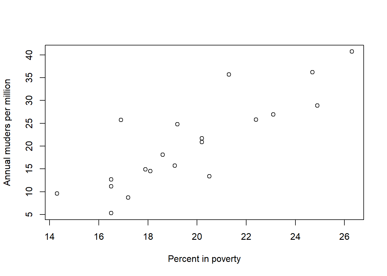
res <- lm(annual_murders_per_mil ~ perc_pov, data = d)
summary(res)
Call:
lm(formula = annual_murders_per_mil ~ perc_pov, data = d)

Residuals:
    Min      1Q  Median      3Q     Max
-9.1663 -2.5613 -0.9552  2.8887 12.3475

Coefficients:
            Estimate Std. Error t value Pr(>|t|)
(Intercept)  -29.901      7.789  -3.839   0.0012 **
perc_pov       2.559      0.390   6.562 3.64e-06 ***
---
Signif. codes:  0 '***' 0.001 '**' 0.01 '*' 0.05 '.' 0.1 ' ' 1

Residual standard error: 5.512 on 18 degrees of freedom
Multiple R-squared:  0.7052,    Adjusted R-squared:  0.6889
F-statistic: 43.06 on 1 and 18 DF,  p-value: 3.638e-06
After fitting the model it is crucial to check whether the model assumptions are valid before performing inference. Assumptions are independency, normality, linearity and constant variance. If there any assumption violation, subsequent inferential procedures may be invalid.
We would also need to investigate unusual observations and whether or not they are influential.
\(\widehat{\mbox{murder}} = -29.901 + 2.559 \mbox{ poverty}\)
\(\hat \beta_0 = -29.901\).
The expected murder rate in metropolitan areas with no poverty is -29.901 per million. This is obviously not a meaningful value, it just serves to adjust the height of the regression line.
\(\hat \beta_1 = 2.559\).
For each additional percentage increase in poverty, we expect the average murders per million to increase 2.559.
\(R^2\) = 0.7052
Poverty levels explains 70.52% of the variability in murder rates in metropolitan areas.
The correlation coefficient is \(r\) = \(\sqrt{R^2} = \sqrt{0.7052}\) = 0.8398.
\(H_0: \beta_1 = 0\)
\(H_1: \beta_1 \neq 0\)
\(\alpha = 0.05\)
\(T = \frac{\hat \beta_1-0}{SE_{\hat \beta_1}} = 6.562\)
p-value is the probability to obtain a test statistic equal to 6.562 or more extreme assuming the null hypothesis is true.
(n <- nrow(d))[1] 202*(1-pt(6.562, n-2))[1] 3.639832e-06p-value is approximately 0. p-value \(< \alpha\), so we reject the null hypothesis.
The data provide convincing evidence that poverty percentage is a significant predictor of murder rate.
95% confidence interval for the slope of poverty percentage
\(2.559 \pm t^* \times SE = 2.559 \pm 2.10 \times 0.390 = (1.740, 3.378)\)
\(t^*\) value such that 0.05/2 probability in t(n-2) is below \(t^*\).
qt(0.025, 20-2)[1] -2.100922c(2.559 - 2.10 * 0.390, 2.559 + 2.10 * 0.390)[1] 1.740 3.378We are 95% confident that for each percentage point poverty is higher, murder rate is expected to be higher on average by 1.74 to 3.378 per million.
The results from the hypothesis test and the confidence interval agree. We rejected the null and the confidence interval does not include 0. In both cases we conclude there is evidence that poverty has an effect on murder rate.
34.1.2 Hospital infection
Consider the hospital infection risk dataset hospital.csv which consists of a sample of n = 58 hospitals in the east and north-central U.S. Conduct a regression analysis for predicting infection risk (percent of patients who get an infection) from average length of stay (in days). In the data, infection risk is variable InfctRsk and average length of stay Stay. Answer the following questions.
- Write out the linear model.
- Interpret the slope.
- What are the hypotheses for evaluating whether lenght of stay is a significant predictor of infection risk? State the conclusion of the hypothesis test in context of the data.
- Interpret \(R^2\).
- Calculate and interpret the mean risk of infection when the average length of stay is 10 days and its standard error.
- Calculate and interpret the confidence interval for the mean risk for an average length of stay of 10 days.
- Calculate and interpret the prediction interval for the mean risk for an average length of stay of 10 days.
- Comment on the difference between confidence and prediction intervals.
Solution
d <- read.csv("data/hospital.csv")
head(d)
ID Stay Age InfctRsk Culture Xray Beds MedSchool Region Census Nurses
1 5 11.20 56.5 5.7 34.5 88.9 180 2 1 134 151
2 10 8.84 56.3 6.3 29.6 82.6 85 2 1 59 66
3 11 11.07 53.2 4.9 28.5 122.0 768 1 1 591 656
4 13 12.78 56.8 7.7 46.0 116.9 322 1 1 252 349
5 18 11.62 53.9 6.4 25.5 99.2 133 2 1 113 101
6 23 9.78 52.3 5.0 17.6 95.9 270 1 1 240 198
Facilities
1 40.0
2 40.0
3 80.0
4 57.1
5 37.1
6 57.1summary(d) ID Stay Age InfctRsk
Min. : 2.00 Min. : 7.390 Min. :38.80 Min. :1.300
1st Qu.: 28.25 1st Qu.: 8.905 1st Qu.:50.60 1st Qu.:3.900
Median : 53.00 Median : 9.930 Median :53.20 Median :4.500
Mean : 52.71 Mean :10.049 Mean :52.78 Mean :4.557
3rd Qu.: 77.75 3rd Qu.:11.060 3rd Qu.:55.60 3rd Qu.:5.300
Max. :109.00 Max. :13.950 Max. :65.90 Max. :7.800
Culture Xray Beds MedSchool
Min. : 2.20 Min. : 42.60 Min. : 52.0 Min. :1.00
1st Qu.:10.65 1st Qu.: 75.95 1st Qu.:133.2 1st Qu.:2.00
Median :16.10 Median : 87.75 Median :195.5 Median :2.00
Mean :18.28 Mean : 86.30 Mean :259.8 Mean :1.81
3rd Qu.:23.62 3rd Qu.: 98.97 3rd Qu.:316.5 3rd Qu.:2.00
Max. :60.50 Max. :133.50 Max. :768.0 Max. :2.00
Region Census Nurses Facilities
Min. :1.000 Min. : 37.0 Min. : 14.0 Min. : 5.70
1st Qu.:1.000 1st Qu.:105.5 1st Qu.: 88.0 1st Qu.:37.10
Median :2.000 Median :159.5 Median :152.0 Median :45.70
Mean :1.552 Mean :198.5 Mean :184.4 Mean :46.01
3rd Qu.:2.000 3rd Qu.:249.0 3rd Qu.:201.5 3rd Qu.:54.30
Max. :2.000 Max. :595.0 Max. :656.0 Max. :80.00 plot(d$InfctRsk, d$Stay,
xlab = "avg length of stay (days)",
ylab = "infection risk (% patients get infection)")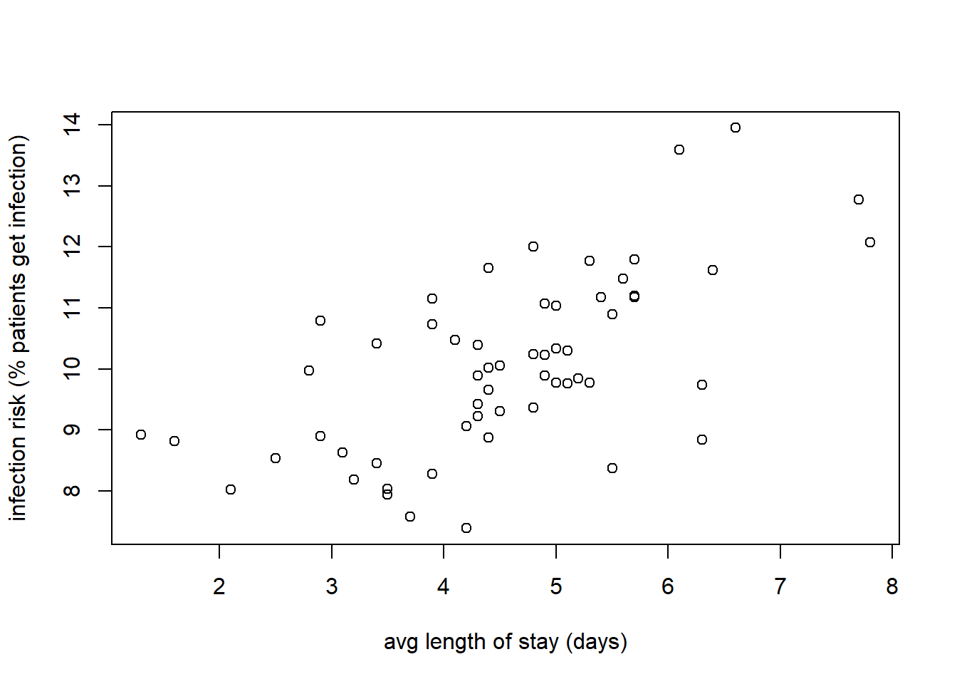
res <- lm(InfctRsk ~ Stay, data = d)
summary(res)
Call:
lm(formula = InfctRsk ~ Stay, data = d)

Residuals:
    Min      1Q  Median      3Q     Max
-2.6145 -0.4660  0.1388  0.4970  2.4310

Coefficients:
            Estimate Std. Error t value Pr(>|t|)
(Intercept) -1.15982    0.95580  -1.213     0.23
Stay         0.56887    0.09416   6.041  1.3e-07 ***
---
Signif. codes:  0 '***' 0.001 '**' 0.01 '*' 0.05 '.' 0.1 ' ' 1

Residual standard error: 1.024 on 56 degrees of freedom
Multiple R-squared:  0.3946,    Adjusted R-squared:  0.3838
F-statistic:  36.5 on 1 and 56 DF,  p-value: 1.302e-07
After fitting the model it is crucial to check whether the model assumptions are valid before performing inference. Assumptions are independency, normality, linearity and constant variance. If there any assumption violation, subsequent inferential procedures may be invalid.
We would also need to investigate unusual observations and whether or not they are influential.
\(\widehat{\mbox{risk}} = -1.15982 + 0.56887 \mbox{ stay}\)
\(\hat \beta_1 = 0.56887\).
We expect the average infection risk to increase 0.56887 for each additional day in the length of stay.
\(H_0: \beta_1 = 0\)
\(H_1: \beta_1 \neq 0\)
\(\alpha = 0.05\)
\(T = \frac{\hat \beta_1-0}{SE_{\hat \beta_1}} = 6.041\)
p-value is the probability to obtain a test statistic equal to 6.041 or more extreme assuming the null hypothesis is true.
(n <- nrow(d))[1] 582*(1-pt(6.041, n-2))[1] 1.303602e-07p-value is approximately 0. p-value \(< \alpha\), so we reject the null hypothesis.
The data provide convincing evidence that length of stay is a significant predictor of infection risk.
\(R^2\) = 0.3946
Length of stay explains 39.46% of the variability in infection risk.
The mean infection risk when the average stay is 10 days is 4.5288.
\(\widehat{\mbox{risk}} = -1.15982 + 0.56887 \times \mbox{ 10} = -1.15982 + 0.56887 \times 10 = 4.5288\)
The standard error of fit \(\widehat{\mbox{risk}}\) measures the accuracy of \(\widehat{\mbox{risk}}\) as an estimate of the mean risk when the average stay is 10 days.
new <- data.frame(Stay = 10)
predict(lm(InfctRsk ~ Stay, data = d), new, interval = "confidence", se.fit = TRUE)
$fit
fit lwr upr
1 4.528846 4.259205 4.798486
$se.fit
[1] 0.1346021
$df
[1] 56
$residual.scale
[1] 1.024489For the 95% CI, we say with 95% confidence we can estimate that in hospitals in which the average length of stay is 10 days, the mean infection risk is between 4.259205 and 4.798486.
new <- data.frame(Stay = 10)
predict(lm(InfctRsk ~ Stay, data = d), new, interval = "confidence", se.fit = TRUE)
$fit
fit lwr upr
1 4.528846 4.259205 4.798486
$se.fit
[1] 0.1346021
$df
[1] 56
$residual.scale
[1] 1.024489We can calculate the 95% CI as
\(\widehat{risk} \pm t^* \times SE(\widehat{risk}) = 4.528846 \pm 2.003241 \times 0.1346021 = (4.259206, 4.798486)\)
c(4.528846 - 2.003241 * 0.1346021, 4.528846 + 2.003241 * 0.1346021)[1] 4.259206 4.798486\(t^*\) is the value such that \(\alpha/2\) probability on the t(n-2) distribution is below \(t^*\).
n <- nrow(d)
qt(0.05/2, n-2)
[1] -2.003241For the 95% PI, we say with 95% confidence that for any future hospital where the average length of stay is 10 days, the infection risk is between 2.45891 and 6.598781.
new <- data.frame(Stay = 10)
predict(lm(InfctRsk ~ Stay, data = d), new, interval = "prediction", se.fit = TRUE)
$fit
fit lwr upr
1 4.528846 2.45891 6.598781
$se.fit
[1] 0.1346021
$df
[1] 56
$residual.scale
[1] 1.024489We can calculate the 95% PI as
\(\widehat{risk} \pm t^* \times \sqrt{MSE + [SE(\widehat{risk})]^2} =\) \(4.528846 \pm 2.003241 \times \sqrt{ 1.024^2 + 0.1346021^2} = (2.459881, 6.597811)\)
c(4.528846 - 2.003241 * sqrt(1.024^2 + 0.1346021^2),
  4.528846 + 2.003241 * sqrt(1.024^2 + 0.1346021^2))
[1] 2.459881 6.597811Residual standard error = \(\sqrt{MSE}\) so MSE = 1.024^2
Note that the formula of the standard error of the prediction is similar to the standard error of the fit when estimating the average risk when stay is 10. The standard error of the prediction just has an extra MSE term added that the standard error of the fit does not.
Prediction intervals are wider than confidence intervals because there is more uncertainty in predicting an individual value of the response variable than in estimating the mean of the response variable.
The formula for the prediction interval has the extra MSE term. A confidence interval for the mean response will always be narrower than the corresponding prediction interval for a new observation.
Furthermore, both intervals are narrowest at the mean of the predictor values.
34.2 Multiple linear regression
34.2.1 Baby weights, Part I
The Child Health and Development Studies investigate a range of topics. One study considered all pregnancies between 1960 and 1967 among women in the Kaiser Foundation Health Plan in the San Francisco East Bay area. Here, we study the relationship between smoking and weight of the baby. The variable smoke is coded 1 if the mother is a smoker, and 0 if not. The summary table below shows the results of a linear regression model for predicting the average birth weight of babies, measured in ounces, based on the smoking status of the mother.
| Estimate | Std. Error | t value | Pr(\(\geq \mid t\mid\)) | |
|---|---|---|---|---|
| (Intercept) | 123.05 | 0.65 | 189.60 | 0.0000 |
| smoke | -8.94 | 1.03 | -8.65 | 0.0000 |
Write the equation of the regression model.
Interpret the slope in this context, and calculate the predicted birth weight of babies born to smoker and non-smoker mothers.
Is there a statistically significant relationship between the average birth weight and smoking?
Solution
\(\widehat{\mbox{weight}} = 123.05 -8.94 \times \mbox{smoke}\)
The estimated body weight of babies born to smoking mothers is 8.94 ounces lower than babies born to non-smoking mothers.
Smoker: \(\widehat{\mbox{weight}} = 123.05 -8.94 \times 1 = 114.11\)
Non-smoker: \(\widehat{\mbox{weight}} = 123.05 -8.94 \times 0 = 123.05\)
\(H_0: \beta_1 = 0\)
\(H_1: \beta_1 \neq 0\)
\(\alpha = 0.05\)
\(T = \frac{\hat \beta_1-0}{SE_{\hat \beta_1}} = -8.65\)
p-value is the probability to obtain a test statistic equal to -8.65 or more extreme assuming the null hypothesis is true.
p-value is approximately 0. p-value \(< \alpha\), so we reject the null hypothesis.
The data provide strong evidence that the true slope parameter is different than 0 and that there is an association between birth weight and smoking. Furthermore, having rejected the null, we can conclude that smoking is associated with lower birth weights.
34.2.2 Baby weights, Part II
The previous exercise Part I introduces a data set on birth weight of babies. Another variable we consider is parity, which is 1 if the child is the first born, and 0 otherwise. The summary table below shows the results of a linear regression model for predicting the average birth weight of babies, measured in ounces, from parity.
| Estimate | Std. Error | t value | Pr(\(\geq \mid t\mid\)) | |
|---|---|---|---|---|
| (Intercept) | 120.07 | 0.60 | 199.94 | 0.0000 |
| parity | -1.93 | 1.19 | -1.62 | 0.1052 |
Write the equation of the regression model.
Interpret the slope in this context, and calculate the predicted birth weight of first borns and others.
Is there a statistically significant relationship between the average birth weight and parity?
Solution
\(\widehat{\mbox{weight}} = 120.07 -1.93 \times \mbox{parity}\)
The estimated body weight of first born babies is 1.93 ounces lower than other babies.
First borns: \(\widehat{\mbox{weight}} = 120.07 - 1.93 \times 1 = 118.14\)
Others: \(\widehat{\mbox{weight}} = 120.07 - 1.93 \times 0 = 120.07\)
\(H_0: \beta_1 = 0\)
\(H_1: \beta_1 \neq 0\)
\(\alpha = 0.05\)
\(T = \frac{\hat \beta_1-0}{SE_{\hat \beta_1}} = -1.62\)
p-value is the probability to obtain a test statistic equal to -1.62 or more extreme assuming the null hypothesis is true.
p-value is 0.1052. p-value \(> \alpha\), so we fail to reject the null hypothesis.
The data do not provide strong evidence that the true slope parameter is different than 0 and that there is an association between birth weight and parity.
34.2.3 Baby weights, Part III
We considered the variables smoke and parity, one at a time, in modeling birth weights of babies in previous exercises Parts I and II. A more realistic approach to modeling infant weights is to consider all possibly related variables at once. Other variables of interest include length of pregnancy in days (gestation), mother’s age in years (age), mother’s height in inches (height), and mother’s pregnancy weight in pounds (weight).
Use the data babies.csv to answer the following questions.
- Write the equation of the regression model that relates birth weights of babies (
bwt) to variablesgestation,parity,age,height,weight, andsmoke. - Interpret the slopes of
gestation,ageandparityin this context. - The coefficient for parity is different than in the linear model shown in exercise Part II. Why might there be a difference?
- Calculate the residual for the first observation in the data set.
- Interpret the adjusted \(R^2\).
Solution
d <- read.csv("data/babies.csv")
head(d)
case bwt gestation parity age height weight smoke
1 1 120 284 0 27 62 100 0
2 2 113 282 0 33 64 135 0
3 3 128 279 0 28 64 115 1
4 4 123 NA 0 36 69 190 0
5 5 108 282 0 23 67 125 1
6 6 136 286 0 25 62 93 0summary(d) case bwt gestation parity
Min. : 1.0 Min. : 55.0 Min. :148.0 Min. :0.0000
1st Qu.: 309.8 1st Qu.:108.8 1st Qu.:272.0 1st Qu.:0.0000
Median : 618.5 Median :120.0 Median :280.0 Median :0.0000
Mean : 618.5 Mean :119.6 Mean :279.3 Mean :0.2549
3rd Qu.: 927.2 3rd Qu.:131.0 3rd Qu.:288.0 3rd Qu.:1.0000
Max. :1236.0 Max. :176.0 Max. :353.0 Max. :1.0000
NA's :13
age height weight smoke
Min. :15.00 Min. :53.00 Min. : 87.0 Min. :0.0000
1st Qu.:23.00 1st Qu.:62.00 1st Qu.:114.8 1st Qu.:0.0000
Median :26.00 Median :64.00 Median :125.0 Median :0.0000
Mean :27.26 Mean :64.05 Mean :128.6 Mean :0.3948
3rd Qu.:31.00 3rd Qu.:66.00 3rd Qu.:139.0 3rd Qu.:1.0000
Max. :45.00 Max. :72.00 Max. :250.0 Max. :1.0000
NA's :2 NA's :22 NA's :36 NA's :10 res <- lm(bwt ~ gestation + parity + age + height + weight + smoke, data = d)
summary(res)
Call:
lm(formula = bwt ~ gestation + parity + age + height + weight +
    smoke, data = d)

Residuals:
    Min      1Q  Median      3Q     Max
-57.613 -10.189  -0.135   9.683  51.713

Coefficients:
             Estimate Std. Error t value Pr(>|t|)
(Intercept) -80.41085   14.34657  -5.605 2.60e-08 ***
gestation     0.44398    0.02910  15.258  < 2e-16 ***
parity       -3.32720    1.12895  -2.947  0.00327 **
age          -0.00895    0.08582  -0.104  0.91696
height        1.15402    0.20502   5.629 2.27e-08 ***
weight        0.05017    0.02524   1.987  0.04711 *
smoke        -8.40073    0.95382  -8.807  < 2e-16 ***
---
Signif. codes:  0 '***' 0.001 '**' 0.01 '*' 0.05 '.' 0.1 ' ' 1

Residual standard error: 15.83 on 1167 degrees of freedom
  (62 observations deleted due to missingness)
Multiple R-squared:  0.258, Adjusted R-squared:  0.2541
F-statistic: 67.61 on 6 and 1167 DF,  p-value: < 2.2e-16
\(\widehat{\mbox{weight}} = -80.41 + 0.44 \mbox{ gestation} - 3.33 \mbox{ parity} -0.01 \mbox{ age} + 1.15 \mbox{ height} + 0.05 \mbox{ weight} -8.40 \mbox{ smoke}\)
\(\hat \beta_{gestation} = 0.44\). The model predicts a 0.44 ounce increase in the birth weight of the baby for each additional day of pregnancy, helding all other covariates constant.
\(\hat \beta_{age} = -0.01\). The model predicts a 0.01 ounce decrease in the birth weight of the baby for each additional year in mothers age, helding all other covariates constant.
\(\hat \beta_{parity} = -3.33\). The model predicts a 3.33 ounce decrease in the birth weight of the baby for first born babies compared to others, helding all other covariates constant.
Parity might be correlated with the other variables in the model, which complicates model estimation.
First observation
d[1, ] case bwt gestation parity age height weight smoke
1 1 120 284 0 27 62 100 0Observed weight = 120
Predicted weight:
\(\widehat{\mbox{weight}} = -80.41 + 0.44 \mbox{284} - 3.33 \mbox{0} -0.01 \mbox{27} + 1.15 \mbox{62} + 0.05 \mbox{100} -8.40 \mbox{0} = 120.58\)
-80.41 + 0.44 * 284 - 3.33 *0 -0.01 *27 + 1.15 *62 + 0.05 *100 -8.40*0[1] 120.58residual = observed weight = predicted weight = 120 - 120.58 = -0.58
The model over-predicts this baby’s birth weight.
R\(^2\)(adj)= 25.41% The percentage of variation explained by the model is about 25% adjusting for the number of parameters.
34.2.4 Cigarette consumption
An insurance organization wanted to study the consumption pattern of cigarettes in all 50 states in the United States and the District of Columbia. The investigators are interested in studying how statewide cigarette consumption is associated with various socioeconomic and demographic variables, and building a parsimonious regression model for predicting the consumption of cigarettes.
The variables for the study are
- Age: Median Age of a person living in the state
- HS: Percentage of people \(>\) 25 years old who completed High School
- Income: Per capita personal income (in dollars)
- Black: Percentage of African Americans
- Female: Percentage of Females
- Price: Weighted average price (in cents) of a pack of cigarettes
- Sales: Number of packs of cigarettes sold
Conduct a regression analysis that can inform investigators how cigarette consumption is associated with the various variables. As part of the analysis, write the regression equation, explain the t tests for coefficients and the F test, interpret R\(^2\)(adj), check assumptions and identify unusual observations. Data are in cigarette.txt.
Solution
d <- read.table("data/cigarette.txt", header = TRUE)
head(d)
State Age HS Income Black Female Price Sales
1 AL 27.0 41.3 2948 26.2 51.7 42.7 89.8
2 AK 22.9 66.7 4644 3.0 45.7 41.8 121.3
3 AZ 26.3 58.1 3665 3.0 50.8 38.5 115.2
4 AR 29.1 39.9 2878 18.3 51.5 38.8 100.3
5 CA 28.1 62.6 4493 7.0 50.8 39.7 123.0
6 CO 26.2 63.9 3855 3.0 50.7 31.1 124.8res <- lm(Sales ~ Age + HS + Income + Black + Female + Price, data = d)
summary(res)
Call:
lm(formula = Sales ~ Age + HS + Income + Black + Female + Price,
    data = d)

Residuals:
    Min      1Q  Median      3Q     Max
-48.398 -12.388  -5.367   6.270 133.213

Coefficients:
             Estimate Std. Error t value Pr(>|t|)
(Intercept) 103.34485  245.60719   0.421  0.67597
Age           4.52045    3.21977   1.404  0.16735
HS           -0.06159    0.81468  -0.076  0.94008
Income        0.01895    0.01022   1.855  0.07036 .
Black         0.35754    0.48722   0.734  0.46695
Female       -1.05286    5.56101  -0.189  0.85071
Price        -3.25492    1.03141  -3.156  0.00289 **
---
Signif. codes:  0 '***' 0.001 '**' 0.01 '*' 0.05 '.' 0.1 ' ' 1

Residual standard error: 28.17 on 44 degrees of freedom
Multiple R-squared:  0.3208,    Adjusted R-squared:  0.2282
F-statistic: 3.464 on 6 and 44 DF,  p-value: 0.006857
Regression equation
\(\widehat{Sales}\) = 103 + 4.52 Age - 0.062 HS + 0.0189 Income + 0.358 Black - 1.05 Female - 3.25 Price
- mean value of sales increases by 4.52 for every unit increase in age, given that the rest of variables remain constant
- mean value of sales decreases by 0.062 for every unit increase in HS, given that the rest of variables remain constant
- mean value of sales increases by 0.0189 for every unit increase in income, given that the rest of variables remain constant
- mean value of sales increases by 0.358 for every unit increase in black, given that the rest of variables remain constant
- mean value of sales decreases by 1.05 for every unit increase in female, given that the rest of variables remain constant
- mean value of sales decreases by 3.25 for every unit increase in price, given that the rest of variables remain constant
Tests for coefficients. t test
Test null hypothesis ‘response variable \(y\) is not linearly related to variable \(x_i\)’ versus alternative hypothesis ‘\(y\) is linearly related to \(x_i\)’, \(i=1,\ldots,p\)
\(H_0\): \(\beta_{i}\) = 0
\(H_1\): \(\beta_{i} \neq 0\)
Test statistic: t-statistic = estimate of the coefficient / SE of coefficient
Distribution: t(n-p-1). t distribution with degrees of freedom = number of observations - number of explanatory variables - 1
p-value: probability of obtaining a test statistic as extreme or more extreme than the one observed
summary(res)
Call:
lm(formula = Sales ~ Age + HS + Income + Black + Female + Price,
    data = d)

Residuals:
    Min      1Q  Median      3Q     Max
-48.398 -12.388  -5.367   6.270 133.213

Coefficients:
             Estimate Std. Error t value Pr(>|t|)
(Intercept) 103.34485  245.60719   0.421  0.67597
Age           4.52045    3.21977   1.404  0.16735
HS           -0.06159    0.81468  -0.076  0.94008
Income        0.01895    0.01022   1.855  0.07036 .
Black         0.35754    0.48722   0.734  0.46695
Female       -1.05286    5.56101  -0.189  0.85071
Price        -3.25492    1.03141  -3.156  0.00289 **
---
Signif. codes:  0 '***' 0.001 '**' 0.01 '*' 0.05 '.' 0.1 ' ' 1

Residual standard error: 28.17 on 44 degrees of freedom
Multiple R-squared:  0.3208,    Adjusted R-squared:  0.2282
F-statistic: 3.464 on 6 and 44 DF, p-value: 0.006857- p-value=0.167, there is not evidence that age affects the mean value of sales allowing for the other predictors.
- p-value=0.940, there is not evidence that HS affects the mean value of sales allowing for the other predictors.
- p-value=0.070, there is some evidence that income affects the mean value of sales allowing for the other predictors.
- p-value=0.467, there is not evidence that black affects the mean value of sales allowing for the other predictors.
- p-value=0.851, there is not evidence that female affects the mean value of sales allowing for the other predictors.
- p-value=0.003, there is strong evidence that price affects the mean value of sales allowing for the other predictors.
ANOVA. F test
Test null hypothesis ‘none of the explanatory variables are useful predictors of the response variable’ versus alternative hypothesis ‘at least one of the explanatory variables is related to the response variable’
\(H_0\): \(\beta_{1} =\beta_{2}=...=\beta_{p}\) = 0
\(H_1\): at least one of \(\beta_1\), \(\beta_2\), \(\dots\), \(\beta_p \neq\) 0
Test statistic: F-statistic = mean squares model / mean squares residual
\[F = \frac{\sum_{i=1}^n (\hat y_i - \bar y)^2/p}{\sum_{i=1}^n ( y_i - \hat y)^2/(n-p-1)} = \frac{SSM/DFM}{SSE/DFE} = \frac{MSM}{MSE},\]
Distribution: F(p, n-p-1). F distribution with degrees of freedom = (number of explanatory variables, number of observations - number of explanatory variables - 1)
p-value: probability that test statistic has a value as extreme or more extreme than the observed
p-value = \(P(F \geq F_{\mbox{observed}})\)
summary(res)
Call:
lm(formula = Sales ~ Age + HS + Income + Black + Female + Price,
    data = d)

Residuals:
    Min      1Q  Median      3Q     Max
-48.398 -12.388  -5.367   6.270 133.213

Coefficients:
             Estimate Std. Error t value Pr(>|t|)
(Intercept) 103.34485  245.60719   0.421  0.67597
Age           4.52045    3.21977   1.404  0.16735
HS           -0.06159    0.81468  -0.076  0.94008
Income        0.01895    0.01022   1.855  0.07036 .
Black         0.35754    0.48722   0.734  0.46695
Female       -1.05286    5.56101  -0.189  0.85071
Price        -3.25492    1.03141  -3.156  0.00289 **
---
Signif. codes:  0 '***' 0.001 '**' 0.01 '*' 0.05 '.' 0.1 ' ' 1

Residual standard error: 28.17 on 44 degrees of freedom
Multiple R-squared:  0.3208,    Adjusted R-squared:  0.2282
F-statistic: 3.464 on 6 and 44 DF,  p-value: 0.006857
p-value=0.007. There is strong evidence that at least one of the explanatory variables in the model is related to the response
R\(^2\)(adj)
R\(^2\)(adj)= 22.82% The percentage of variation explained by the model is about 23% adjusting for the number of parameters.
summary(res)$adj.r.squared[1] 0.2282303Check assumptions
- Independence
Random sample
- Normality
To check normality we look at the normal Q-Q plot of the residuals. The data show departure from normality because the points do not form a straight line.
plot(res, 2)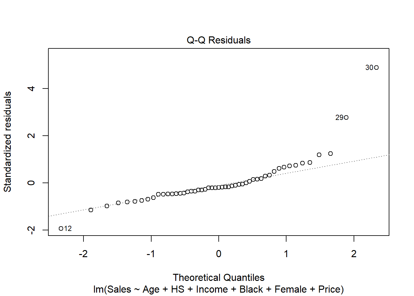
- Linearity and constant variance
Linearity. Residual versus variables plots indicate that the effect of the explanatory variables may not be linear.
Constant variance. Points are not randomly scattered around 0. The assumption of constance variance of \(y\), \(\sigma^2\), for all values of \(x\) does not hold.
par(mfrow = c(2, 3))
plot(d$Age, rstandard(res))
abline(h = 0, lty = 2)
plot(d$HS, rstandard(res))
abline(h = 0, lty = 2)
plot(d$Income, rstandard(res))
abline(h = 0, lty = 2)
plot(d$Black, rstandard(res))
abline(h = 0, lty = 2)
plot(d$Female, rstandard(res))
abline(h = 0, lty = 2)
plot(d$Price, rstandard(res))
abline(h = 0, lty = 2)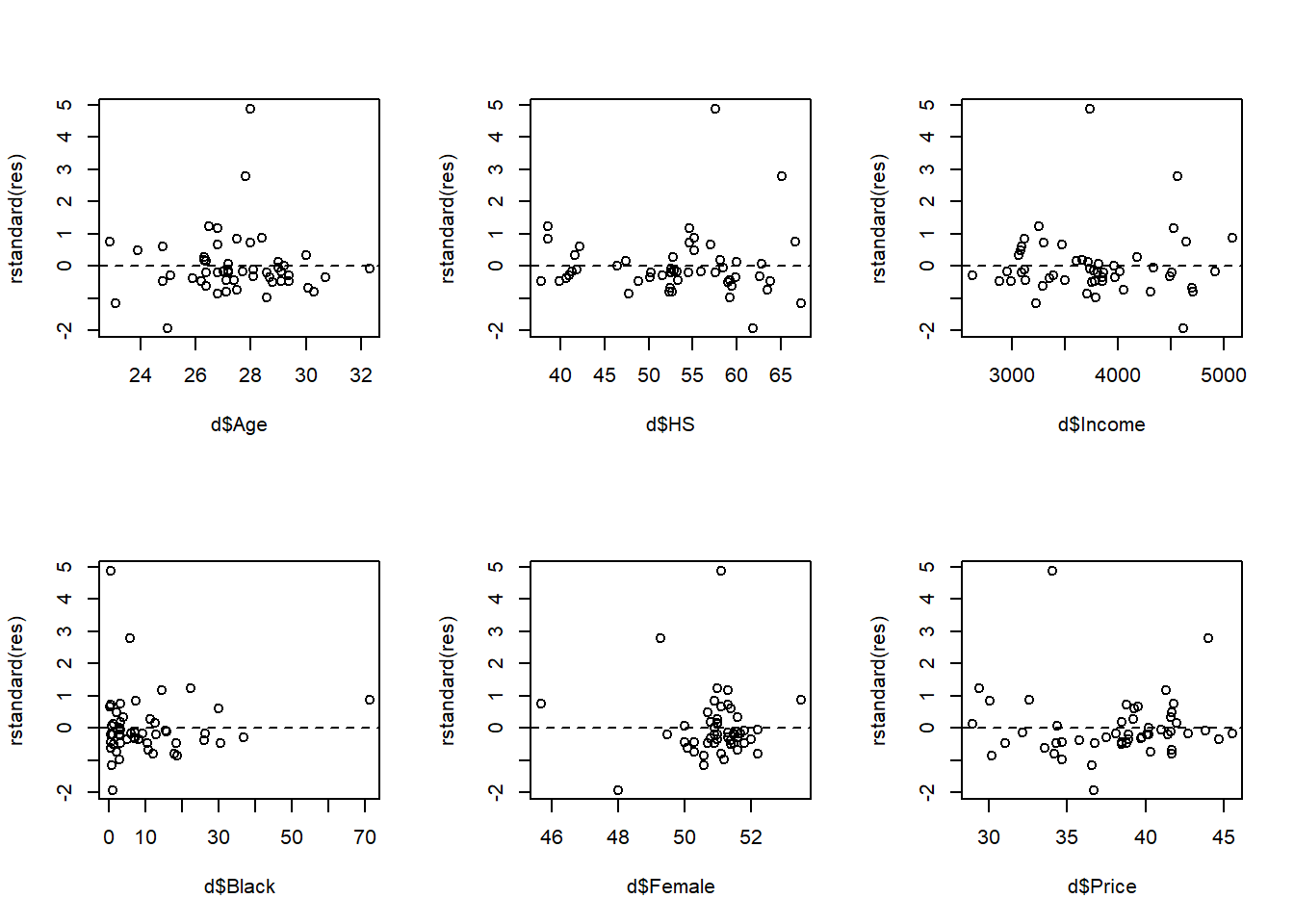
Unusual observations
Outliers (unusual \(y\)). Standardized residuals less than -2 or greater than 2.
# Outliers
op <- which(abs(rstandard(res)) > 2)
op
29 30
29 30 High leverage observations (unusual \(x\)). Leverage greater than 2 times the average of all leverage values. That is, \(h_{ii} > 2(p+1)/n\).
# High leverage observations
h <- hatvalues(res)
lp <- which(h > 2*length(res$coefficients)/nrow(d))
lp
2 9 10 45
2 9 10 45 Influential values. Cook’s distance higher than \(4/n\).
# Influential observations
ip <- which(cooks.distance(res) > 4/nrow(d))
ip
2 9 12 29 30 45
2 9 12 29 30 45 plot(res, 4)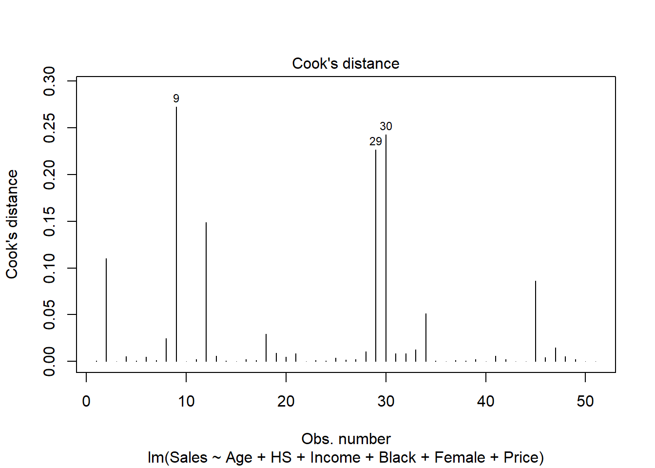
d[unique(c(lp, op, ip)), ] State Age HS Income Black Female Price Sales
2 AK 22.9 66.7 4644 3.0 45.7 41.8 121.3
9 DC 28.4 55.2 5079 71.1 53.5 32.6 200.4
10 FL 32.3 52.6 3738 15.3 51.8 43.8 123.6
45 UT 23.1 67.3 3227 0.6 50.6 36.6 65.5
29 NV 27.8 65.2 4563 5.7 49.3 44.0 189.5
30 NH 28.0 57.6 3737 0.3 51.1 34.1 265.7
12 HI 25.0 61.9 4623 1.0 48.0 36.7 82.1- Outliers: observations with large residual: 29, 30
- High leverage observations: observations with large unusual value of explanatory variables: 2, 9, 10, 45
- Observation 9 has a very high percentage of African Americans in DC. Is it a data entry error?
- Influential observations: observations 2, 9, 12, 29, 30 and 45 may be affecting the analysis too much. We would need to omit these observations, run the analysis without them and see how they impact the results.