31 Generalized Additive Models (GAMs)
31.1 Generalized Additive Models (GAMs)
Chapter 7.7 Generalized Additive Models: PDF Book Statistical Learning R
A natural way to extend the multiple regression model
\[y_i = \beta_0 + \beta_1 x_{i1} + \beta_2 x_{i2} + \ldots + \beta_p x_{ip} + \epsilon_i\]
in order to allow for non-linear relationships between each covariate and the response is to replace each linear component \(\beta_j x_{ij}\) with a (smooth) non-linear function \(f_j(x_{ij})\).
\[y_i = \beta_0 + \sum_{i=1}^p f_j(x_{ij}) + \epsilon_i = \beta_0 + f_1(x_{i1}) + f(x_{i2}) + \ldots + f(x_{ip}) + \epsilon_i\] This is an example of a GAM. It is called an additive model because we calculate a separate \(f_j\) for each \(X_j\) , and then add together all of their contributions.
We do not have to use splines as the building blocks for GAMs: we can just as well use local regression, polynomial regression, or any combination of the approaches seen earlier in this chapter in order to create a GAM.
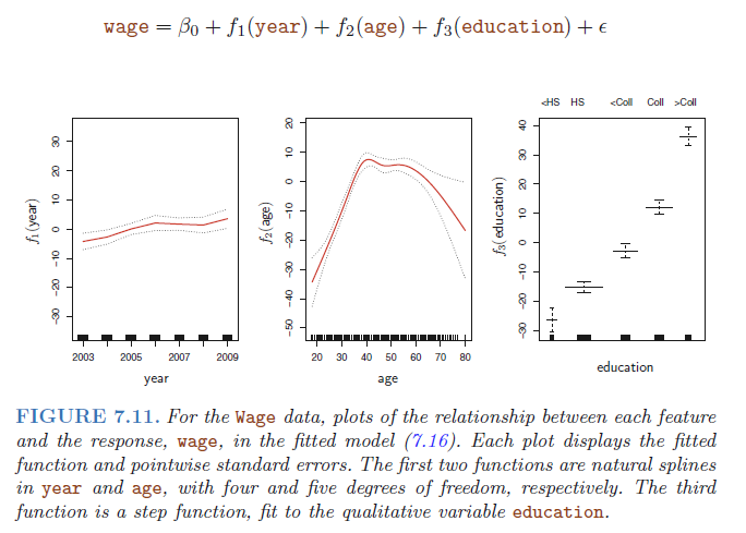
Figure 7.11 shows the results of fitting the model using least squares. This is easy to do, since natural splines can be constructed using an appropriately chosen set of basis functions. Hence the entire model is just a big regression onto spline basis variables and dummy variables, all packed into one big regression matrix.
The left-hand panel indicates that holding age and education fixed, wage tends to increase slightly with year; this may be due to inflation. The center panel indicates that holding education and year fixed, wage tends to be highest for intermediate values of age, and lowest for the very young and very old. The right-hand panel indicates that holding year and age fixed, wage tends to increase with education: the more educated a person is, the higher their salary, on average.
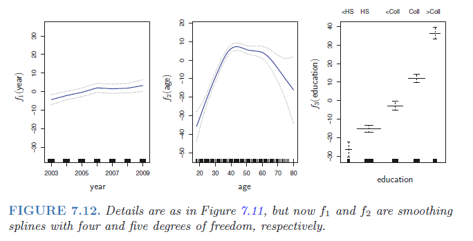
Figure 7.12 shows a similar triple of plots, but this time f1 and f2 are smoothing splines with four and five degrees of freedom, respectively. Fitting a GAM with a smoothing spline is not quite as simple as fitting a GAM with a natural spline, since in the case of smoothing splines, least squares cannot be used. However, standard software such as the gam() function in R can be used to fit GAMs using smoothing splines, via an approach known as backfitting.
The fitted functions in Figures 7.11 and 7.12 look rather similar. In most situations, the differences in the GAMs obtained using smoothing splines versus natural splines are small.
31.2 R packages for fitting GAMs
Chapter 15 Additive Models: PDF Book Faraway
There are several different ways of fitting additive models in R. The gam package originates from the work of Hastie and Tibshirani (1990). The mgcv package is part of the recommended suite that comes with the default installation of R and is based on methods described in Wood (2000).
The gam package allows more choice in the smoothers used while the mgcv package has an automatic choice in the amount of smoothing as well as wider functionality.
31.3 Fitting algorithms
31.3.1 Backfitting algorithm
The fitting algorithm depends on the package used. The backfitting algorithm is used in the gam package.
We initialize by setting \(\beta_0 = \bar y\) and \(f_j(x) = \hat \beta_j x\) where \(\hat \beta_j\) is some initial estimate, such as the least squares, for \(j=1,\ldots,p\)
We cycle \(j=1,\ldots,p,1,\ldots,p,1,\ldots\)
\[f_j = S(x_j, y - \beta_0 - \sum_{i \neq j} f_i(X_i))\] where \(S(x,y)\) means the smooth on the data \((x,y)\). The choice of S is left open to the user. It could be a nonparametric smoother like splines or loess, or it could be a parametric fit, say linear or polynomial. We can even use different smoothers on different predictors with differing amounts of smoothing.
- The algorithm is iterated until convergence.
The term \(y- \beta_0 - \sum_{i \neq j} f_i(X_i)\) is a partial residual - the result of fitting everything except \(x_j\).
For example, a partial residual for \(X_3\) has the form \(r_i = y_i − f_1(x_{i1}) − f_2(x_{i2})\). If we know \(f_1\) and \(f_2\), then we can fit \(f_3\) by treating this residual as a response in a non-linear regression on \(X_3\).
31.3.2 Penalized smoothing spline approach
The mgcv package employs a penalized smoothing spline approach. Suppose we represent
\[f_j(x)=\sum_i \beta_i \phi_i(x)\] for a family of spline basis functions \(\phi_i\). We impose a penalty \[\int [f''_j(x)]^2 dx\] which can be written in the form \(\beta_j ' S_j \beta_j\), for a suitable matrix \(S_j\) that depends on the chose of basis. We then maximize:
\[log L(\beta) - \sum_j \lambda_j \beta_j' S_j \beta_j\] where \(L(\beta)\) is likelihood with respect to \(\beta\) and the \(\lambda_j\)s control the amount of smoothing for each variable. Generalized cross-validation (GCV) is used to select the \(\lambda_j\)s.
31.4 Examples
Lab 7.8.3 GAMs: PDF Book Statistical Learning R
Chapter 15.1 Modeling Ozone Concentration: PDF Book Faraway
Chapter 7.4 Air pollution in Chicago (distributed lag non-linear models): PDF Book Generalized Additive Models